# Creating Your Own Functions {#sec-functions}
```{r}
#| label: setup-ch16
#| include: false
library(tidyverse)
```
::: {.callout-note}
## Learning Objectives
By the end of this chapter, you will be able to:
- Write functions with flexible argument handling
- Use default arguments and `...` (dots) to pass arguments
- Understand R's lexical scoping rules
- Use `stopifnot()` and `tryCatch()` for error handling
- Debug functions using `browser()` and `debug()`
:::
## Why Write Functions? {#sec-why-functions}
The rule of thumb: if you copy-paste a block of code more than twice, it belongs in a function. Functions:
1. **Reduce repetition** — change the logic in one place, not many
2. **Name operations** — a good function name is self-documenting
3. **Enable testing** — isolated functions can be tested systematically
4. **Enable reuse** — in other scripts or packages
## Function Syntax {#sec-syntax}
```{r}
#| label: basic-function
# General form
# function_name <- function(arg1, arg2 = default) {
# body
# return(value) # or just the last expression
# }
# A simple example
standardise <- function(x) {
(x - mean(x, na.rm = TRUE)) / sd(x, na.rm = TRUE)
}
standardise(c(10, 20, 30, 40, 50))
# With default arguments
describe_variable <- function(x, digits = 2, na.rm = TRUE) {
tibble(
n = length(x),
missing = sum(is.na(x)),
mean = round(mean(x, na.rm = na.rm), digits),
sd = round(sd(x, na.rm = na.rm), digits),
min = min(x, na.rm = na.rm),
max = max(x, na.rm = na.rm)
)
}
describe_variable(airquality$Ozone)
describe_variable(airquality$Ozone, digits = 1)
```
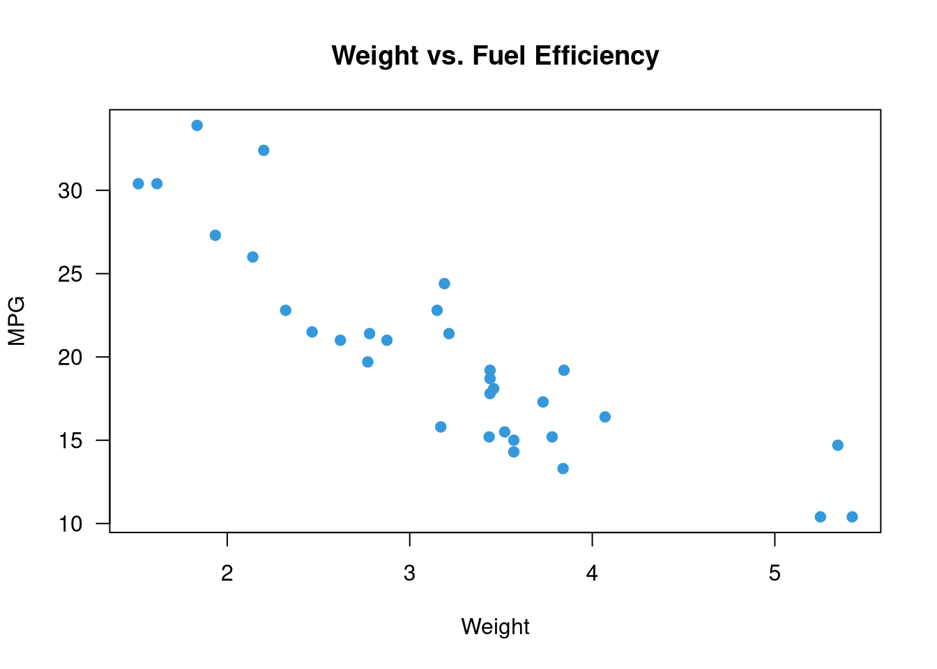
## The Dots (`...`) Argument {#sec-dots}
`...` allows a function to accept arbitrary additional arguments and pass them on:
```{r}
#| label: dots-demo
# Pass ... to an inner function
nice_plot <- function(x, y, ...) {
  plot(x, y,
       pch = 19,
       col = "#3498db",
       las = 1,
       ...)   # Any additional plot() arguments are passed through
}

nice_plot(mtcars$wt, mtcars$mpg,
          xlab = "Weight", ylab = "MPG",
          main = "Weight vs. Fuel Efficiency")
```
## Input Validation {#sec-validation}
Good functions check their inputs:
```{r}
#| label: validation
compute_ci <- function(x, conf = 0.95, na.rm = TRUE) {
# Input validation
if (!is.numeric(x))
stop("`x` must be a numeric vector", call. = FALSE)
if (length(conf) != 1 || conf <= 0 || conf >= 1)
stop("`conf` must be a single number between 0 and 1", call. = FALSE)
if (na.rm) x <- x[!is.na(x)]
n <- length(x)
alpha <- 1 - conf
se <- sd(x) / sqrt(n)
t_val <- qt(1 - alpha / 2, df = n - 1)
list(
mean = mean(x),
lower = mean(x) - t_val * se,
upper = mean(x) + t_val * se,
conf = conf
)
}
compute_ci(airquality$Temp)
# compute_ci("not numeric") # Error: x must be numeric
```
## Scope and Environments {#sec-scope}
R uses **lexical scoping**: a function looks for variables in the environment where it was *defined*, not where it was *called*.
```{r}
#| label: scope-demo
x <- 10 # Global variable
add_to_x <- function(y) {
x + y # Uses x from the global environment
}
add_to_x(5) # 15
# Local variables don't leak out
my_func <- function() {
local_var <- 42
local_var
}
my_func()
# local_var # Error: object 'local_var' not found
```
## Error Handling {#sec-error-handling}
```{r}
#| label: error-handling
# tryCatch: handle errors, warnings, and messages gracefully
safe_log <- function(x) {
tryCatch(
expr = log(x),
warning = function(w) {
message("Warning: ", conditionMessage(w))
NA_real_
},
error = function(e) {
message("Error: ", conditionMessage(e))
NA_real_
}
)
}
safe_log(10) # Works
safe_log(-1) # Returns NA with warning
safe_log("hello") # Returns NA with error message
# purrr::safely wraps any function to return list(result, error)
safe_sqrt <- purrr::safely(sqrt)
safe_sqrt(4)
safe_sqrt("abc")
```
## Debugging {#sec-debugging}
```{r}
#| eval: false
# browser(): pauses execution inside a function
buggy_function <- function(x) {
  result <- x * 2
  browser()           # Pauses here — you can inspect the environment
  result + some_typo  # This will error
}

# debug(): set a function to always enter browser mode
debug(buggy_function)
buggy_function(5)   # Enters browser mode

# traceback(): after an error, shows the call stack
f <- function(x) g(x)
g <- function(x) log(x)
# f("a")       # Error
# traceback()  # Shows which functions were in the call stack
```
## A Case Study: A Reusable EDA Function {#sec-function-case-study}
```{r}
#| label: eda-function
#' Compute a tidy summary of a numeric variable by group
#'
#' @param df A data frame
#' @param var The numeric variable to summarise (unquoted)
#' @param group The grouping variable (unquoted)
#' @param digits Number of decimal places
#' @return A tibble with summary statistics per group
group_summary <- function(df, var, group, digits = 2) {
# Validate
if (!is.data.frame(df)) stop("`df` must be a data frame")
var_name <- deparse(substitute(var))
group_name <- deparse(substitute(group))
if (!var_name %in% names(df))
stop(paste0("Column '", var_name, "' not found in data frame"))
df |>
group_by({{ group }}) |>
summarise(
n = n(),
missing = sum(is.na({{ var }})),
mean = round(mean({{ var }}, na.rm = TRUE), digits),
median = round(median({{ var }}, na.rm = TRUE), digits),
sd = round(sd({{ var }}, na.rm = TRUE), digits),
q25 = round(quantile({{ var }}, 0.25, na.rm = TRUE), digits),
q75 = round(quantile({{ var }}, 0.75, na.rm = TRUE), digits),
.groups = "drop"
)
}
# Usage
group_summary(gapminder::gapminder |> filter(year == 2007),
var = lifeExp,
group = continent)
```
## Exercises {#sec-ch16-exercises}
1. Write a function `winsorise(x, lower = 0.05, upper = 0.95)` that replaces extreme values with the 5th and 95th percentiles. Test it on a vector with obvious outliers.
2. Write a function `multiple_regression_summary(df, outcome, predictors)` that fits a linear model and returns a tidy coefficient table with confidence intervals.
3. Add input validation to the function in Exercise 2: check that the outcome and all predictors exist as columns, that the outcome is numeric, and that there are enough observations.
4. Demonstrate R's lexical scoping: write two functions with the same local variable name. Show they don't interfere with each other.
5. **Challenge:** Write a function `batch_report(data_dir, output_dir)` that reads all `.csv` files in a directory, applies your `group_summary()` function, and writes one summary CSV per input file to the output directory. Use `purrr::walk()`.