# Hypothesis Testing {#sec-hypothesis}
```{r}
#| label: setup-ch8
#| include: false
library(tidyverse)
set.seed(42)
```
::: {.callout-note}
## Learning Objectives
By the end of this chapter, you will be able to:
- State the logic and vocabulary of null hypothesis significance testing
- Perform one-sample, two-sample, and paired t-tests in R
- Apply non-parametric alternatives when assumptions are violated
- Conduct chi-squared tests for categorical data
- Interpret p-values correctly and avoid common misinterpretations
:::
## The Logic of Hypothesis Testing {#sec-logic}
**Null Hypothesis Significance Testing (NHST)** follows a specific logic:
1. State the **null hypothesis** H₀ (the "nothing going on" hypothesis)
2. State the **alternative hypothesis** H₁ (what you expect to find)
3. Choose a **significance level** α (typically 0.05)
4. Compute a **test statistic** from the data
5. Compute the **p-value**: P(data this extreme | H₀ is true)
6. If p < α, **reject H₀**; otherwise, **fail to reject H₀**
::: {.callout-important}
## What a p-value Is NOT
- It is **not** the probability that H₀ is true
- It is **not** the probability that your result occurred by chance
- A p-value > 0.05 does **not** mean H₀ is true
- A small p-value does **not** mean the effect is practically important
A p-value is: *P(observing data this extreme, assuming H₀ is true).*
:::
## Parametric Tests {#sec-parametric}
### One-Sample t-test {#sec-one-sample-t}
**Question:** Is the mean yield of our wheat variety significantly different from the national average of 4500 kg/ha?
```{r}
#| label: one-sample-t
set.seed(42)
farm_yields <- rnorm(35, mean = 4800, sd = 680)
# H₀: μ = 4500
# H₁: μ ≠ 4500 (two-tailed)
result <- t.test(farm_yields, mu = 4500, alternative = "two.sided")
print(result)
# One-tailed: test if our variety EXCEEDS the average
t.test(farm_yields, mu = 4500, alternative = "greater")
```
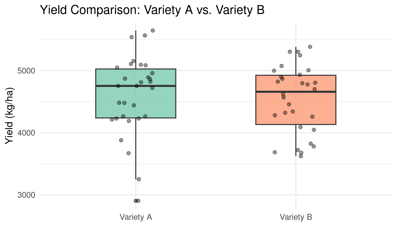
### Two-Sample t-test (Independent) {#sec-two-sample-t}
**Question:** Do two varieties (A and B) have different mean yields?
```{r}
#| label: two-sample-t
variety_A <- rnorm(30, mean = 4700, sd = 600)
variety_B <- rnorm(30, mean = 4400, sd = 650)
# First: check if variances are equal (Levene's test)
library(car)
var.test(variety_A, variety_B) # F-test for equal variances
# Welch t-test (does not assume equal variances — default in R)
t.test(variety_A, variety_B, var.equal = FALSE)
# Student t-test (assumes equal variances)
t.test(variety_A, variety_B, var.equal = TRUE)
```
```{r}
#| label: fig-two-sample
#| fig-cap: "Distribution of yields for Variety A and Variety B."
#| fig-width: 7
#| fig-height: 4
tibble(
  yield   = c(variety_A, variety_B),
  variety = rep(c("Variety A", "Variety B"), each = 30)
) |>
  ggplot(aes(x = variety, y = yield, fill = variety)) +
  geom_boxplot(alpha = 0.7, width = 0.5) +
  geom_jitter(width = 0.15, alpha = 0.4) +
  scale_fill_brewer(palette = "Set2") +
  labs(title = "Yield Comparison: Variety A vs. Variety B",
       x = NULL, y = "Yield (kg/ha)") +
  theme_minimal(base_size = 13) +
  theme(legend.position = "none")
```
### Paired t-test {#sec-paired-t}
Use when observations come in pairs — e.g., measuring the same field before and after treatment.
```{r}
#| label: paired-t
set.seed(10)
before_treatment <- rnorm(25, mean = 3200, sd = 400)
after_treatment <- before_treatment + rnorm(25, mean = 350, sd = 200)
# Paired t-test
t.test(after_treatment, before_treatment, paired = TRUE)
# Equivalent to one-sample t-test on the differences
differences <- after_treatment - before_treatment
t.test(differences, mu = 0)
```
## Non-Parametric Tests {#sec-nonparametric}
Non-parametric tests make fewer distributional assumptions and are appropriate when:
- The data are clearly non-normal and n is small
- Data are ordinal (ranked)
- Outliers are present and cannot be removed
### Mann-Whitney U Test (Wilcoxon Rank-Sum) {#sec-mann-whitney}
The non-parametric alternative to the independent two-sample t-test:
```{r}
#| label: mann-whitney
# Simulate non-normal data
group_1 <- rexp(25, rate = 1/5) # Right-skewed
group_2 <- rexp(25, rate = 1/7) # Different rate
wilcox.test(group_1, group_2, alternative = "two.sided")
```
### Wilcoxon Signed-Rank Test {#sec-wilcoxon-signed}
The non-parametric alternative to the paired t-test:
```{r}
#| label: wilcoxon-signed
wilcox.test(after_treatment, before_treatment, paired = TRUE)
```
### Kruskal-Wallis Test {#sec-kruskal-wallis}
The non-parametric alternative to one-way ANOVA (for comparing 3+ groups):
```{r}
#| label: kruskal-wallis
soil_pH <- tibble(
pH = c(rnorm(20, 6.2, 0.4), rnorm(20, 6.8, 0.5), rnorm(20, 7.1, 0.3)),
group = rep(c("Sandy", "Loam", "Clay"), each = 20)
)
kruskal.test(pH ~ group, data = soil_pH)
# Post-hoc: pairwise Wilcoxon with correction
pairwise.wilcox.test(soil_pH$pH, soil_pH$group, p.adjust.method = "BH")
```
## Chi-Squared Tests {#sec-chi-squared}
### Goodness of Fit {#sec-chi-gof}
Tests whether observed frequencies match expected frequencies:
```{r}
#| label: chi-gof
# Observed die rolls
observed <- c(15, 18, 12, 20, 17, 18) # 100 rolls, 6 sides
expected_probs <- rep(1/6, 6) # Expected under fair die
chisq.test(observed, p = expected_probs)
```
### Test of Independence {#sec-chi-independence}
Tests whether two categorical variables are independent:
```{r}
#| label: chi-independence
# Contingency table: crop adoption by state
adoption_table <- matrix(
c(45, 30, 25, 60, 20, 40, 35, 55, 10),
nrow = 3,
dimnames = list(
State = c("Punjab", "Haryana", "UP"),
Adoption = c("Improved Seeds", "Traditional", "Mixed")
)
)
print(adoption_table)
result_chi <- chisq.test(adoption_table)
print(result_chi)
# Expected counts (should be > 5 for chi-sq to be valid)
result_chi$expected
# Standardised residuals (which cells drive the result?)
round(result_chi$stdres, 2)
```
## Effect Sizes {#sec-effect-size}
Statistical significance tells you *whether* an effect exists; **effect size** tells you *how large* it is.
```{r}
#| label: effect-sizes
library(effectsize)
# Cohen's d for t-tests
cohens_d(variety_A, variety_B)
# Interpretation: small=0.2, medium=0.5, large=0.8
# Eta-squared for chi-squared
cramers_v(adoption_table)
```
## Multiple Testing {#sec-multiple-testing}
When you run many tests, false positives accumulate. With 20 tests at α=0.05, you expect one false positive by chance.
```{r}
#| label: multiple-testing
# Raw p-values
p_values <- c(0.01, 0.04, 0.08, 0.15, 0.03, 0.22, 0.001)
# Bonferroni correction (conservative)
p.adjust(p_values, method = "bonferroni")
# Benjamini-Hochberg (less conservative, controls false discovery rate)
p.adjust(p_values, method = "BH")
```
## Exercises {#sec-ch8-exercises}
1. The national average daily caloric intake is 2100 kcal. A survey of 45 households in a tribal district finds a mean of 1850 kcal (SD = 320). Test whether this district has significantly lower caloric intake than the national average. State H₀, H₁, and your conclusion clearly.
2. Two groups of farmers are given different training programs. After 6 months, their yield improvements are measured. Test whether the programs differ in effectiveness. Check the assumption of equal variances first.
3. Using `airquality`, test whether ozone levels are significantly different between May and August. First check whether the data are normally distributed (use `shapiro.test()`). Choose the appropriate test based on the result.
4. Create a 3×2 contingency table of a categorical variable of your choice and test for independence using a chi-squared test. Compute Cramér's V to interpret the strength of association.
5. **Challenge:** Perform a simulation study to demonstrate the multiple testing problem. Generate 1000 datasets of 20 uncorrelated variables. Run pairwise t-tests. What proportion of results are "significant" at α=0.05? How does Bonferroni correction help?