12 Time Series Analysis

Learning Objectives

By the end of this chapter, you will be able to:

Create and manipulate time series objects in R
Decompose a time series into trend, seasonal, and remainder components
Test for stationarity using the ADF test
Fit ARIMA models using auto.arima()
Produce and visualise forecasts with confidence intervals

12.1 Time Series Objects

Code

# Base R ts object: monthly retail sales (simulated)
set.seed(99)
monthly_sales <- ts(
  data      = round(1000 + seq(0, 200, length.out = 60) +    # Trend
                    100 * sin(2 * pi * (1:60) / 12) +         # Seasonality
                    rnorm(60, 0, 40)),                         # Noise
  start     = c(2019, 1),    # January 2019
  frequency = 12             # Monthly
)

print(monthly_sales)
#>       Jan  Feb  Mar  Apr  May  Jun  Jul  Aug  Sep  Oct  Nov  Dec
#> 2019 1059 1109 1110 1115 1049 1022  936  957  913  892  954 1074
#> 2020 1121 1030 1026 1137 1088  988 1031  989 1012 1015 1022 1064
#> 2021 1140 1193 1215 1156 1090 1154 1107 1036 1003 1030  973 1064
#> 2022 1164 1215 1232 1232 1191 1072 1081  997  994 1012 1069 1125
#> 2023 1279 1247 1206 1284 1239 1164 1090 1097 1069 1122 1119 1170

Code

autoplot(monthly_sales) +
  labs(title = "Monthly Retail Sales (Simulated)",
       x = "Year", y = "Sales (₹ thousands)") +
  theme_minimal(base_size = 13)

Figure 12.1: Monthly retail sales time series with trend and seasonal patterns.

12.2 Time Series Decomposition

12.2.1 Classical Decomposition

Code

decomp <- stl(monthly_sales, s.window = "periodic")

autoplot(decomp) +
  labs(title = "STL Decomposition of Monthly Sales") +
  theme_minimal(base_size = 12)

Figure 12.2: STL decomposition separating trend, seasonality, and remainder.

Code

# Extract components
trend     <- decomp$time.series[, "trend"]
seasonal  <- decomp$time.series[, "seasonal"]
remainder <- decomp$time.series[, "remainder"]

# Seasonal strength
var(seasonal) / (var(seasonal) + var(remainder))
#> [1] 0.8217406

12.3 Stationarity

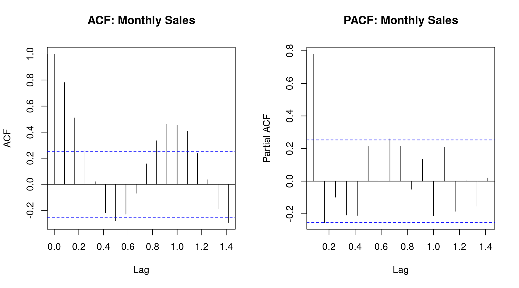
Most time series models require stationarity — constant mean, variance, and autocovariance over time.

Code

par(mfrow = c(1, 2))
acf(monthly_sales, main = "ACF: Monthly Sales")
pacf(monthly_sales, main = "PACF: Monthly Sales")
par(mfrow = c(1, 1))

Figure 12.3: ACF and PACF plots help identify appropriate ARIMA orders.

Code

library(tseries)

# Augmented Dickey-Fuller test
# H₀: series has a unit root (non-stationary)
# H₁: series is stationary
adf.test(monthly_sales)
#> 
#>  Augmented Dickey-Fuller Test
#> 
#> data:  monthly_sales
#> Dickey-Fuller = -5.5889, Lag order = 3, p-value = 0.01
#> alternative hypothesis: stationary

# If non-stationary, differencing can help
adf.test(diff(monthly_sales))
#> 
#>  Augmented Dickey-Fuller Test
#> 
#> data:  diff(monthly_sales)
#> Dickey-Fuller = -3.5618, Lag order = 3, p-value = 0.04412
#> alternative hypothesis: stationary

12.4 ARIMA Models

ARIMA(p, d, q) models combine: - AR(p): Autoregressive — depends on p past values - I(d): Integrated — d-th order differencing for stationarity - MA(q): Moving average — depends on q past errors

For seasonal data, use SARIMA(p, d, q)(P, D, Q)[m].

Code

# auto.arima selects the best model automatically
m_arima <- auto.arima(
  monthly_sales,
  seasonal     = TRUE,
  stepwise     = FALSE,
  approximation = FALSE
)

summary(m_arima)
#> Series: monthly_sales 
#> ARIMA(0,0,1)(1,1,0)[12] with drift 
#> 
#> Coefficients:
#>          ma1     sar1   drift
#>       0.5171  -0.6805  3.2357
#> s.e.  0.1399   0.1161  0.5353
#> 
#> sigma^2 = 2103:  log likelihood = -254.07
#> AIC=516.14   AICc=517.07   BIC=523.63
#> 
#> Training set error measures:
#>                      ME     RMSE      MAE       MPE     MAPE      MASE
#> Training set -0.4338316 39.71361 30.15103 -0.142812 2.743794 0.5121194
#>                     ACF1
#> Training set -0.02565537

Code

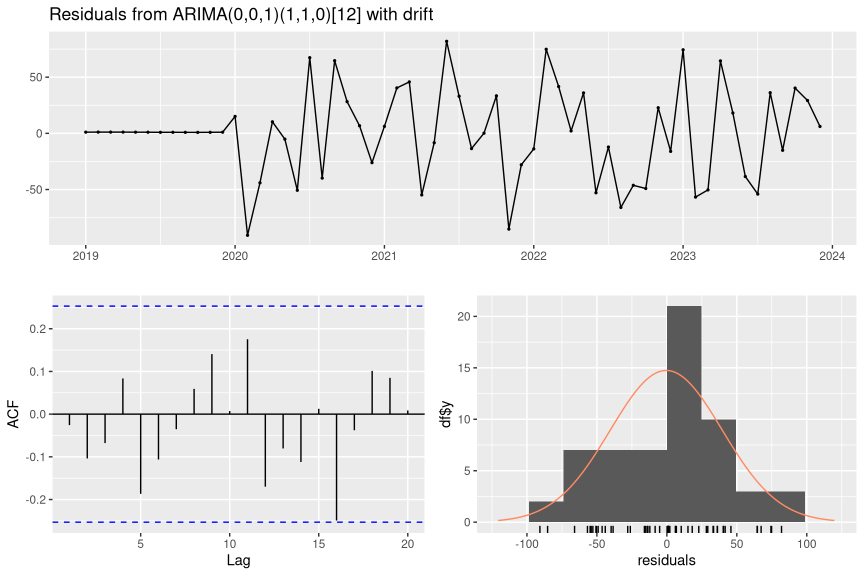
checkresiduals(m_arima)
#> 
#>  Ljung-Box test
#> 
#> data:  Residuals from ARIMA(0,0,1)(1,1,0)[12] with drift
#> Q* = 10.991, df = 10, p-value = 0.3582
#> 
#> Model df: 2.   Total lags used: 12

Figure 12.4: ARIMA model residual diagnostics.

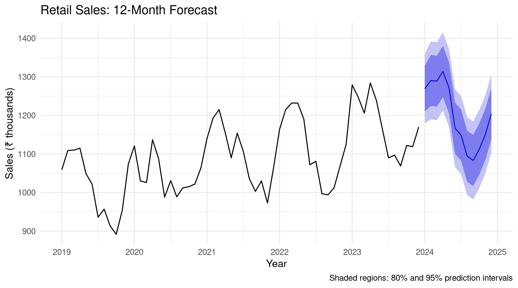
12.5 Forecasting

Code

forecast_result <- forecast(m_arima, h = 12)

autoplot(forecast_result) +
  labs(title = "Retail Sales: 12-Month Forecast",
       x = "Year", y = "Sales (₹ thousands)",
       caption = "Shaded regions: 80% and 95% prediction intervals") +
  theme_minimal(base_size = 13)

Figure 12.5: 12-month ahead forecast with 80% and 95% prediction intervals.

Code

# Hold-out validation: train on first 48 months, test on last 12
train  <- head(monthly_sales, 48)
test   <- tail(monthly_sales, 12)

m_train <- auto.arima(train, seasonal = TRUE)
fc      <- forecast(m_train, h = 12)

# Accuracy metrics
accuracy(fc, test)
#>                      ME     RMSE      MAE        MPE     MAPE      MASE
#> Training set -0.3323314 37.26928 27.09198 -0.1320103 2.534815 0.4707100
#> Test set      7.4850869 47.88616 41.11243  0.5669466 3.472503 0.7143086
#>                    ACF1 Theil's U
#> Training set 0.03242358        NA
#> Test set     0.09449067 0.8920096

12.6 The tsibble Framework

For modern, tidy time series workflows:

Code

library(tsibble)
library(feasts)

# Convert to tsibble
sales_tsibble <- as_tsibble(monthly_sales)

# Decompose
sales_tsibble |>
  model(STL(value ~ trend(window = 13) + season(window = "periodic"))) |>
  components() |>
  autoplot() +
  theme_minimal(base_size = 11) +
  labs(title = "STL Decomposition (tsibble/feasts)")

12.7 Exercises

Download monthly diesel or petrol price data for India from the PPAC website. Import and convert to a ts object. Plot the series and describe the trend and any seasonality.
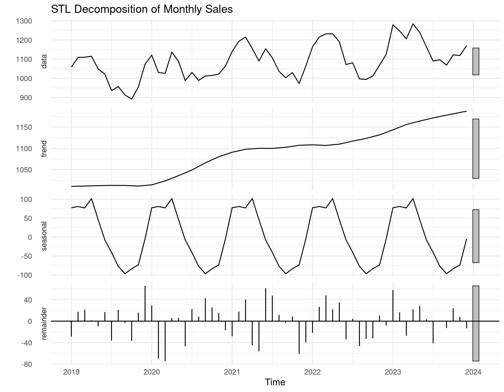
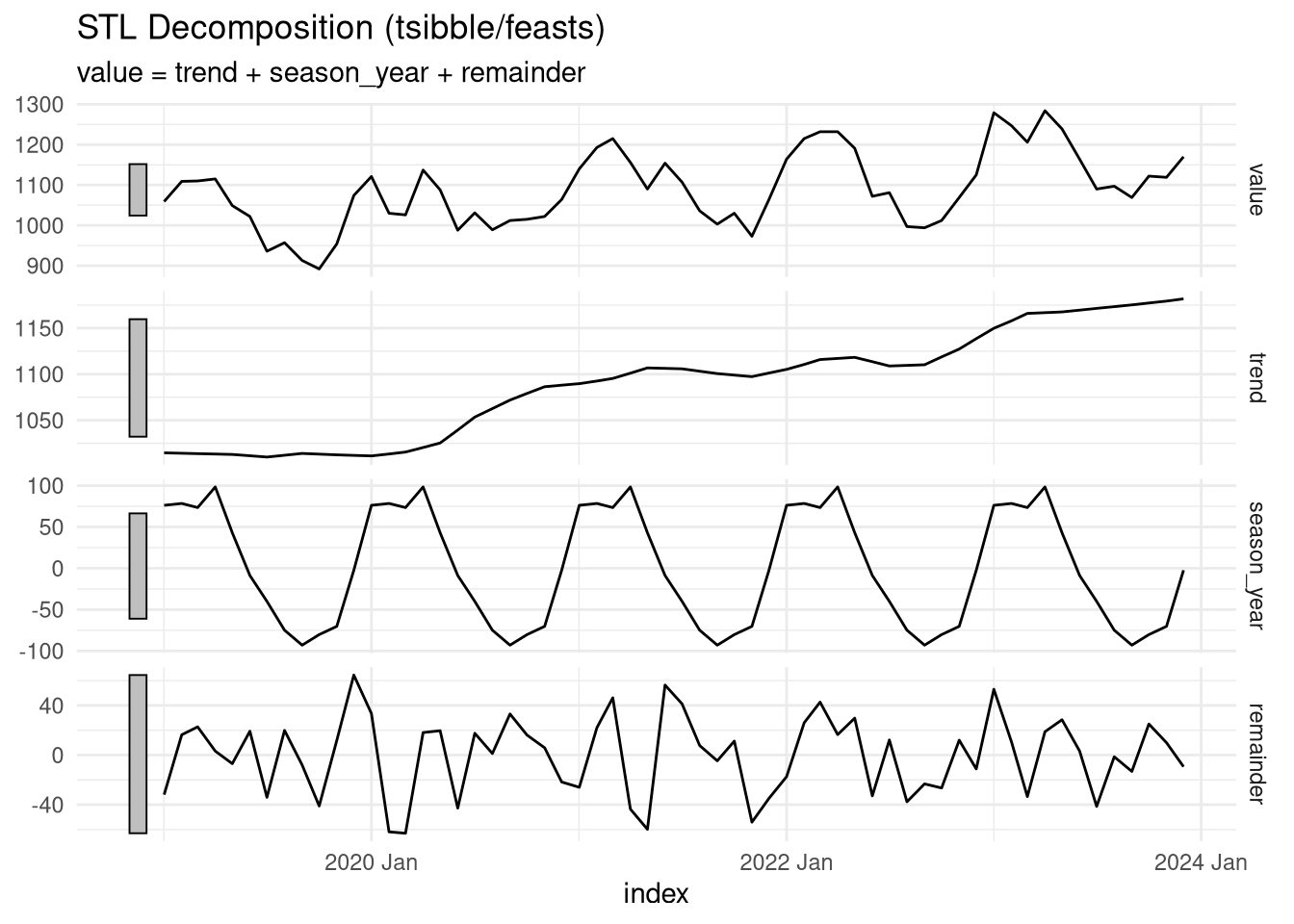
Decompose the price series using STL. Plot the components and estimate the seasonal strength.
Fit an ARIMA model using auto.arima(). Print the selected order and the model summary.
Produce a 24-month forecast. Visualise it and write a brief interpretation of the projection.
Challenge: Build a comparison of three forecasting methods — Exponential Smoothing, ARIMA, and a linear trend model — evaluated by out-of-sample RMSE on a holdout set of 12 months.

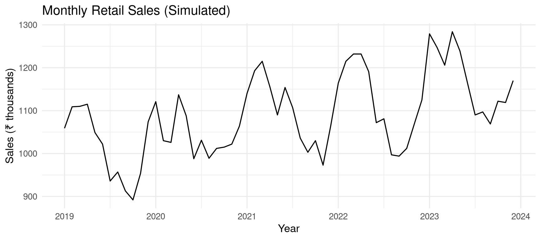
# Time Series Analysis {#sec-timeseries} ```{r} #| label: setup-ch14 #| include: false library(tidyverse) library(forecast) library(tsibble) library(feasts) set.seed(42) ``` ::: {.callout-note} ## Learning Objectives By the end of this chapter, you will be able to: - Create and manipulate time series objects in R - Decompose a time series into trend, seasonal, and remainder components - Test for stationarity using the ADF test - Fit ARIMA models using `auto.arima()` - Produce and visualise forecasts with confidence intervals ::: ## Time Series Objects {#sec-ts-objects} ```{r} #| label: ts-create # Base R ts object: monthly retail sales (simulated) set.seed(99) monthly_sales <- ts( data = round(1000 + seq(0, 200, length.out = 60) + # Trend 100 * sin(2 * pi * (1:60) / 12) + # Seasonality rnorm(60, 0, 40)), # Noise start = c(2019, 1), # January 2019 frequency = 12 # Monthly ) print(monthly_sales) ``` ```{r} #| label: fig-ts-plot #| fig-cap: "Monthly retail sales time series with trend and seasonal patterns." #| fig-width: 9 #| fig-height: 4 autoplot(monthly_sales) + labs(title = "Monthly Retail Sales (Simulated)", x = "Year", y = "Sales (₹ thousands)") + theme_minimal(base_size = 13) ``` ## Time Series Decomposition {#sec-decomposition} ### Classical Decomposition {#sec-classical-decomp} ```{r} #| label: fig-decomp #| fig-cap: "STL decomposition separating trend, seasonality, and remainder." #| fig-width: 9 #| fig-height: 7 decomp <- stl(monthly_sales, s.window = "periodic") autoplot(decomp) + labs(title = "STL Decomposition of Monthly Sales") + theme_minimal(base_size = 12) ``` ```{r} #| label: decomp-extract # Extract components trend <- decomp$time.series[, "trend"] seasonal <- decomp$time.series[, "seasonal"] remainder <- decomp$time.series[, "remainder"] # Seasonal strength var(seasonal) / (var(seasonal) + var(remainder)) ``` ## Stationarity {#sec-stationarity} Most time series models require **stationarity** — constant mean, variance, and autocovariance over time. ```{r} #| label: fig-acf-pacf #| fig-cap: "ACF and PACF plots help identify appropriate ARIMA orders." #| fig-width: 9 #| fig-height: 5 par(mfrow = c(1, 2)) acf(monthly_sales, main = "ACF: Monthly Sales") pacf(monthly_sales, main = "PACF: Monthly Sales") par(mfrow = c(1, 1)) ``` ```{r} #| label: stationarity-test library(tseries) # Augmented Dickey-Fuller test # H₀: series has a unit root (non-stationary) # H₁: series is stationary adf.test(monthly_sales) # If non-stationary, differencing can help adf.test(diff(monthly_sales)) ``` ## ARIMA Models {#sec-arima} **ARIMA(p, d, q)** models combine: - **AR(p):** Autoregressive — depends on p past values - **I(d):** Integrated — d-th order differencing for stationarity - **MA(q):** Moving average — depends on q past errors For seasonal data, use **SARIMA(p, d, q)(P, D, Q)[m]**. ```{r} #| label: arima-fit # auto.arima selects the best model automatically m_arima <- auto.arima( monthly_sales, seasonal = TRUE, stepwise = FALSE, approximation = FALSE ) summary(m_arima) ``` ```{r} #| label: fig-arima-diag #| fig-cap: "ARIMA model residual diagnostics." #| fig-width: 9 #| fig-height: 6 checkresiduals(m_arima) ``` ## Forecasting {#sec-forecasting} ```{r} #| label: fig-forecast #| fig-cap: "12-month ahead forecast with 80% and 95% prediction intervals." #| fig-width: 9 #| fig-height: 5 forecast_result <- forecast(m_arima, h = 12) autoplot(forecast_result) + labs(title = "Retail Sales: 12-Month Forecast", x = "Year", y = "Sales (₹ thousands)", caption = "Shaded regions: 80% and 95% prediction intervals") + theme_minimal(base_size = 13) ``` ```{r} #| label: forecast-accuracy # Hold-out validation: train on first 48 months, test on last 12 train <- head(monthly_sales, 48) test <- tail(monthly_sales, 12) m_train <- auto.arima(train, seasonal = TRUE) fc <- forecast(m_train, h = 12) # Accuracy metrics accuracy(fc, test) ``` ## The tsibble Framework {#sec-tsibble} For modern, tidy time series workflows: ```{r} #| label: tsibble-demo library(tsibble) library(feasts) # Convert to tsibble sales_tsibble <- as_tsibble(monthly_sales) # Decompose sales_tsibble |> model(STL(value ~ trend(window = 13) + season(window = "periodic"))) |> components() |> autoplot() + theme_minimal(base_size = 11) + labs(title = "STL Decomposition (tsibble/feasts)") ``` ## Exercises {#sec-ch14-exercises} 1. Download monthly diesel or petrol price data for India from the PPAC website. Import and convert to a `ts` object. Plot the series and describe the trend and any seasonality. 2. Decompose the price series using STL. Plot the components and estimate the seasonal strength. 3. Fit an ARIMA model using `auto.arima()`. Print the selected order and the model summary. 4. Produce a 24-month forecast. Visualise it and write a brief interpretation of the projection. 5. **Challenge:** Build a comparison of three forecasting methods — Exponential Smoothing, ARIMA, and a linear trend model — evaluated by out-of-sample RMSE on a holdout set of 12 months.