# Generalized Linear Models {#sec-glm}
```{r}
#| label: setup-ch11
#| include: false
library(tidyverse)
library(broom)
library(modelsummary)
set.seed(42)
```
::: {.callout-note}
## Learning Objectives
By the end of this chapter, you will be able to:
- Explain why linear regression fails for binary and count outcomes
- Fit and interpret logistic regression models
- Compute and interpret odds ratios
- Fit Poisson regression for count data
- Assess model fit with deviance and AIC
:::
## Why GLMs? {#sec-why-glm}
Linear regression assumes the outcome is continuous and normally distributed. Many real outcomes violate this:
- **Binary outcomes** (yes/no, success/failure) → Logistic Regression
- **Count outcomes** (number of events, hospital visits) → Poisson Regression
- **Rate outcomes** (events per person-year) → Poisson with offset
**Generalized Linear Models (GLMs)** unify these cases through:
1. A **distribution** (Normal, Binomial, Poisson, ...)
2. A **link function** connecting the linear predictor to the outcome mean
## Logistic Regression {#sec-logistic}
For a binary outcome $Y \in \{0, 1\}$, we model the log-odds:
$$\log\left(\frac{p}{1-p}\right) = \beta_0 + \beta_1 X_1 + \cdots + \beta_k X_k$$
```{r}
#| label: logistic-data
# Simulate: probability of adopting improved seeds depends on education and income
set.seed(42)
n <- 300
farm_data <- tibble(
education_yrs = round(rnorm(n, mean = 8, sd = 3), 0) |> pmax(0),
income_lakh = round(runif(n, 1, 15), 1),
access_market = rbinom(n, 1, 0.6)
) |>
mutate(
log_odds = -3.5 + 0.25 * education_yrs + 0.12 * income_lakh + 0.8 * access_market,
prob = plogis(log_odds),
adopted = rbinom(n, 1, prob)
)
table(farm_data$adopted)
mean(farm_data$adopted)
```
```{r}
#| label: logistic-fit
m_logit <- glm(
adopted ~ education_yrs + income_lakh + access_market,
data = farm_data,
family = binomial(link = "logit")
)
summary(m_logit)
```
### Interpreting Logistic Regression {#sec-logistic-interpretation}
Raw coefficients are in **log-odds**, which are hard to interpret. We exponentiate to get **odds ratios**:
```{r}
#| label: odds-ratios
# Tidy with confidence intervals
tidy_logit <- tidy(m_logit, exponentiate = TRUE, conf.int = TRUE)
print(tidy_logit)
```
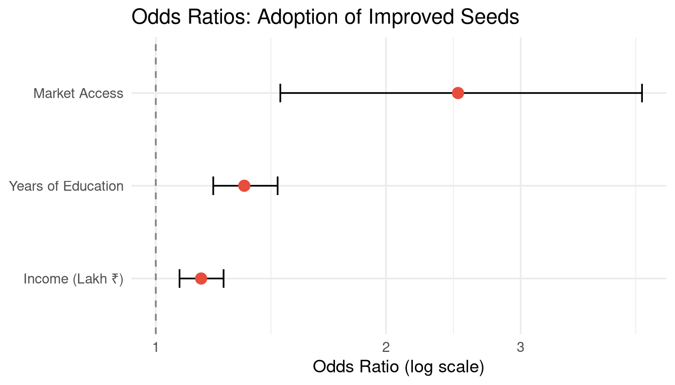
```{r}
#| label: fig-odds-ratios
#| fig-cap: "Odds ratios with 95% confidence intervals for adoption of improved seeds."
#| fig-width: 7
#| fig-height: 4
tidy_logit |>
  filter(term != "(Intercept)") |>
  mutate(term = recode(term,
                       "education_yrs" = "Years of Education",
                       "income_lakh"   = "Income (Lakh ₹)",
                       "access_market" = "Market Access")) |>
  ggplot(aes(x = estimate, y = reorder(term, estimate))) +
  geom_vline(xintercept = 1, linetype = "dashed", colour = "grey50") +
  geom_errorbarh(aes(xmin = conf.low, xmax = conf.high), height = 0.2) +
  geom_point(size = 3.5, colour = "#e74c3c") +
  scale_x_log10() +
  labs(title = "Odds Ratios: Adoption of Improved Seeds",
       x = "Odds Ratio (log scale)", y = NULL) +
  theme_minimal(base_size = 13)
```
::: {.callout-tip}
## Interpreting Odds Ratios
- **OR = 1**: No association
- **OR > 1**: Predictor increases the odds of the outcome
- **OR < 1**: Predictor decreases the odds of the outcome
"Farmers with market access have `r round(tidy_logit$estimate[tidy_logit$term == "access_market"], 2)` times the odds of adopting improved seeds, compared to those without market access, holding other variables constant."
:::
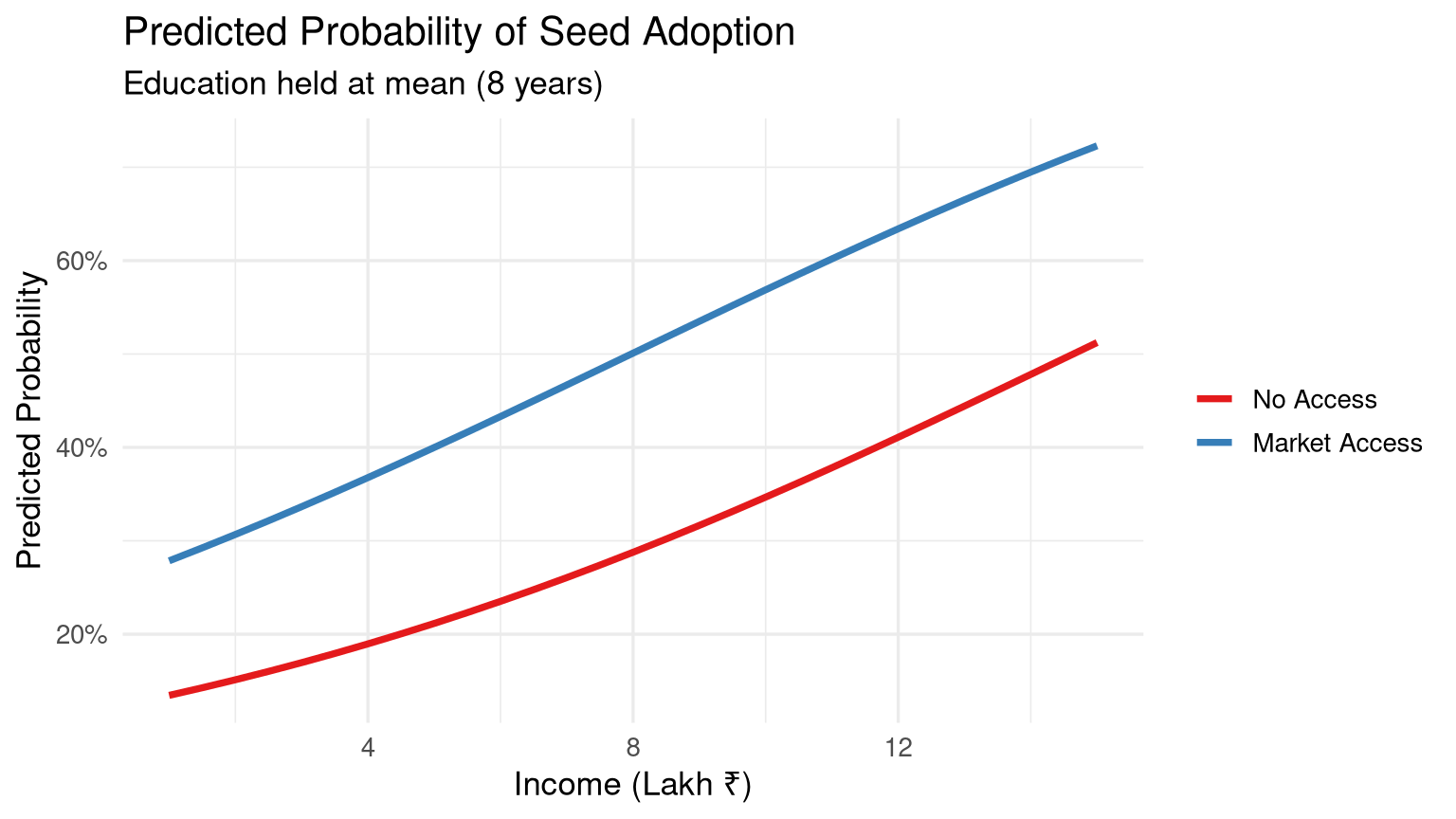
### Predicted Probabilities {#sec-predicted-probs}
```{r}
#| label: fig-predicted-probs
#| fig-cap: "Predicted probability of seed adoption by income level and market access."
#| fig-width: 8
#| fig-height: 4.5
# Create prediction grid
pred_grid <- expand_grid(
  income_lakh   = seq(1, 15, by = 0.5),
  access_market = c(0, 1),
  education_yrs = mean(farm_data$education_yrs)
) |>
  mutate(
    pred_prob = predict(m_logit, newdata = pick(everything()), type = "response"),
    market    = factor(access_market, labels = c("No Access", "Market Access"))
  )

ggplot(pred_grid, aes(x = income_lakh, y = pred_prob, colour = market)) +
  geom_line(linewidth = 1.3) +
  scale_colour_brewer(palette = "Set1") +
  labs(title   = "Predicted Probability of Seed Adoption",
       subtitle = paste0("Education held at mean (", round(mean(farm_data$education_yrs), 1), " years)"),
       x = "Income (Lakh ₹)", y = "Predicted Probability", colour = NULL) +
  scale_y_continuous(labels = scales::percent_format()) +
  theme_minimal(base_size = 13)
```
### Model Fit {#sec-logistic-fit}
```{r}
#| label: logistic-fit-stats
# Null and residual deviance
glance(m_logit)
# McFadden's pseudo R-squared
mcfadden_r2 <- 1 - (m_logit$deviance / m_logit$null.deviance)
cat("McFadden R²:", round(mcfadden_r2, 3), "\n")
# Classification accuracy
threshold <- 0.5
predicted_class <- as.integer(fitted(m_logit) >= threshold)
conf_matrix <- table(Predicted = predicted_class, Actual = farm_data$adopted)
print(conf_matrix)
accuracy <- mean(predicted_class == farm_data$adopted)
cat("Accuracy:", round(accuracy * 100, 1), "%\n")
```
## Poisson Regression {#sec-poisson-reg}
For count outcomes (non-negative integers), Poisson regression models the log of the expected count:
$$\log(\mu_i) = \beta_0 + \beta_1 X_{1i} + \cdots$$
```{r}
#| label: poisson-data
# Hospital admissions per month in different districts
set.seed(7)
hospital_data <- tibble(
district = rep(paste("District", 1:30), each = 12),
month = rep(1:12, 30),
n_admissions = rpois(360, lambda = exp(2.8 + 0.04 * rep(1:12, 30))),
temperature = round(15 + 10 * sin(2 * pi * (1:360) / 12) + rnorm(360, 0, 2), 1),
urban = rbinom(360, 1, 0.4)
)
head(hospital_data)
```
```{r}
#| label: poisson-fit
m_poisson <- glm(
n_admissions ~ temperature + urban + factor(month),
data = hospital_data,
family = poisson(link = "log")
)
# Exponentiated coefficients are Incidence Rate Ratios (IRR)
tidy(m_poisson, exponentiate = TRUE, conf.int = TRUE) |>
filter(!str_detect(term, "month")) |>
select(term, estimate, conf.low, conf.high, p.value)
```
### Checking for Overdispersion {#sec-overdispersion}
A key assumption of Poisson regression is that the mean equals the variance. When the variance exceeds the mean (**overdispersion**), use negative binomial regression instead.
```{r}
#| label: overdispersion-check
# Dispersion test
dispersion_ratio <- sum(residuals(m_poisson, type = "pearson")^2) / m_poisson$df.residual
cat("Dispersion ratio:", round(dispersion_ratio, 3),
"\n(Values >> 1 indicate overdispersion)\n")
# If overdispersed, use negative binomial
library(MASS)
m_negbin <- MASS::glm.nb(n_admissions ~ temperature + urban, data = hospital_data)
```
## Regression Table: All Models {#sec-glm-table}
```{r}
#| label: tbl-glm-comparison
#| tbl-cap: "Summary of GLM specifications. Logistic uses odds ratios; Poisson uses IRR."
modelsummary(
  list("Logistic (Adoption)" = m_logit, "Poisson (Admissions)" = m_poisson),
  exponentiate = TRUE,
  stars        = TRUE,
  gof_map      = c("nobs", "AIC", "BIC"),
  coef_omit    = "month"
)
```
## Exercises {#sec-ch11-exercises}
1. Using the `Titanic` dataset (or `titanic` package), fit a logistic regression predicting survival as a function of passenger class, sex, and age. Interpret the odds ratios. Who had the best survival odds?
2. Simulate a count outcome (e.g., number of pest-infested fields) as a function of rainfall and temperature. Fit a Poisson regression and interpret the incidence rate ratios.
3. Test your Poisson model from Exercise 2 for overdispersion. If overdispersion is present, fit a negative binomial model and compare AIC values.
4. For a logistic regression model, explain in plain language the difference between: (a) a coefficient in log-odds, (b) an odds ratio, and (c) a predicted probability.
5. **Challenge:** Using India's National Family Health Survey (NFHS) data, model the binary outcome of child vaccination (full immunisation yes/no) as a function of mother's education, wealth index, and place of residence (urban/rural). Create a coefficient plot and write a policy-relevant interpretation.