# Linear Regression Models {#sec-regression}
```{r}
#| label: setup-ch10
#| include: false
library(tidyverse)
library(broom)
library(modelsummary)
library(car)
set.seed(42)
```
::: {.callout-note}
## Learning Objectives
By the end of this chapter, you will be able to:
- Fit and interpret simple and multiple linear regression models using `lm()`
- Understand and evaluate R-squared and adjusted R-squared
- Read regression diagnostic plots and identify problems
- Check for multicollinearity using Variance Inflation Factors
- Present clean regression tables using `modelsummary`
:::
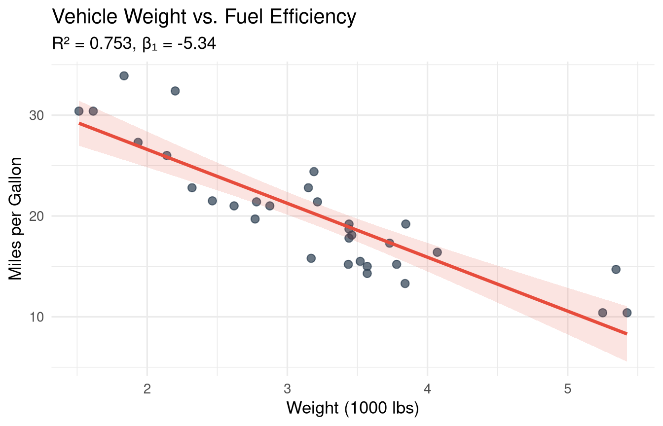
## Simple Linear Regression {#sec-slr}
**Simple linear regression** models the relationship between one predictor (X) and one outcome (Y):
$$Y_i = \beta_0 + \beta_1 X_i + \varepsilon_i, \quad \varepsilon_i \sim N(0, \sigma^2)$$
```{r}
#| label: slr-data
data(mtcars)
# Research question: Does car weight predict fuel efficiency?
m_slr <- lm(mpg ~ wt, data = mtcars)
summary(m_slr)
```
```{r}
#| label: fig-slr
#| fig-cap: "Simple linear regression: fuel efficiency decreases with vehicle weight."
#| fig-width: 7
#| fig-height: 4.5
ggplot(mtcars, aes(x = wt, y = mpg)) +
  geom_point(size = 2.5, colour = "#2c3e50", alpha = 0.7) +
  geom_smooth(method = "lm", se = TRUE, colour = "#e74c3c",
              fill = "#e74c3c", alpha = 0.15) +
  labs(
    title    = "Vehicle Weight vs. Fuel Efficiency",
    subtitle = sprintf("R² = %.3f, β₁ = %.2f",
                       summary(m_slr)$r.squared,
                       coef(m_slr)[2]),
    x = "Weight (1000 lbs)",
    y = "Miles per Gallon"
  ) +
  theme_minimal(base_size = 13)
```
### Interpreting Coefficients {#sec-slr-interpretation}
```{r}
#| label: slr-interpretation
coef(m_slr)
confint(m_slr, level = 0.95)
```
**Intercept (β₀ = `r round(coef(m_slr)[1], 2)`):** The predicted MPG when weight = 0 (not meaningful here — extrapolation).
**Slope (β₁ = `r round(coef(m_slr)[2], 2)`):** For each additional 1000 lbs of weight, MPG decreases by `r abs(round(coef(m_slr)[2], 2))` units on average.
**R² = `r round(summary(m_slr)$r.squared, 3)`:** `r round(summary(m_slr)$r.squared * 100, 1)`% of the variation in MPG is explained by weight.
### Predictions {#sec-predictions}
```{r}
#| label: predictions
# Predict MPG for new weight values
new_cars <- data.frame(wt = c(2.0, 3.0, 4.0, 5.0))
predict(m_slr, newdata = new_cars, interval = "confidence") # CI for mean
predict(m_slr, newdata = new_cars, interval = "prediction") # PI for individual
```
## Multiple Linear Regression {#sec-mlr}
When we add more predictors:
$$Y_i = \beta_0 + \beta_1 X_{1i} + \beta_2 X_{2i} + \cdots + \beta_k X_{ki} + \varepsilon_i$$
```{r}
#| label: mlr-model
# Add horsepower and number of cylinders as predictors
m_mlr <- lm(mpg ~ wt + hp + factor(cyl), data = mtcars)
summary(m_mlr)
```
### Comparing Models {#sec-model-comparison}
```{r}
#| label: model-comparison
# Nested model comparison with F-test
m1 <- lm(mpg ~ wt, data = mtcars)
m2 <- lm(mpg ~ wt + hp, data = mtcars)
m3 <- lm(mpg ~ wt + hp + factor(cyl), data = mtcars)
anova(m1, m2, m3)
# AIC and BIC (lower = better)
AIC(m1, m2, m3)
BIC(m1, m2, m3)
```
### Regression Tables with `modelsummary` {#sec-reg-tables}
```{r}
#| label: tbl-regression
#| tbl-cap: "Regression models predicting fuel efficiency (MPG)."
modelsummary(
  list("Model 1" = m1, "Model 2" = m2, "Model 3" = m3),
  stars      = TRUE,
  gof_map    = c("nobs", "r.squared", "adj.r.squared", "AIC"),
  coef_rename = c(
    "(Intercept)"   = "Intercept",
    "wt"            = "Weight",
    "hp"            = "Horsepower",
    "factor(cyl)6"  = "6 Cylinders",
    "factor(cyl)8"  = "8 Cylinders"
  ),
  notes = "Standard errors in parentheses. *, **, *** = 10%, 5%, 1% significance."
)
```
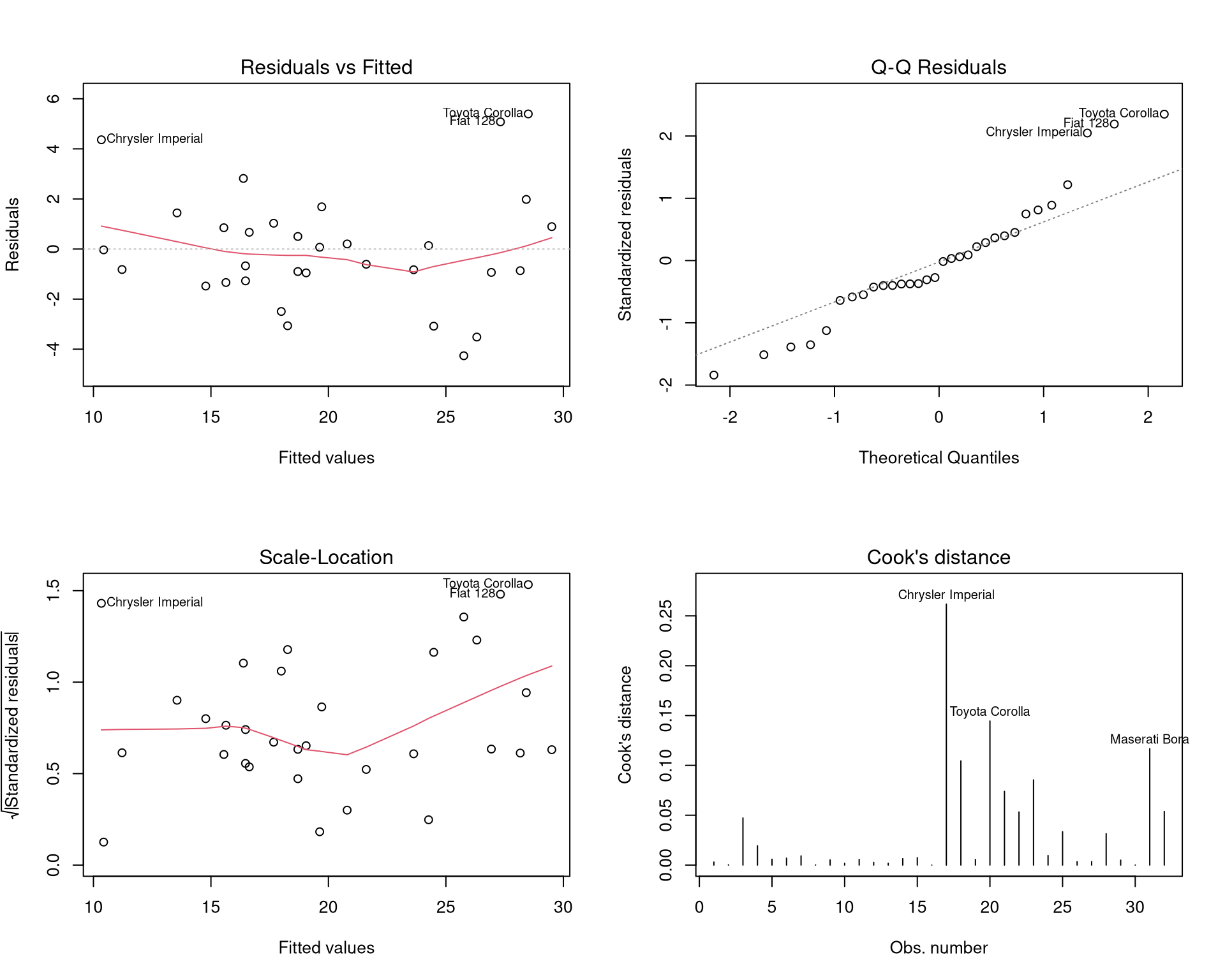
## Regression Diagnostics {#sec-diagnostics}
Linear regression requires four key assumptions: **L**inearity, **I**ndependence, **N**ormality of residuals, **E**qual variance (LINE).
```{r}
#| label: fig-diagnostics
#| fig-cap: "Regression diagnostic plots for the multiple regression model."
#| fig-width: 10
#| fig-height: 8
par(mfrow = c(2, 2))
plot(m_mlr, which = 1:4)
par(mfrow = c(1, 1))
```
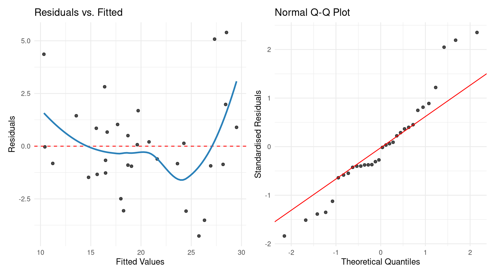
### Residuals vs. Fitted {#sec-residuals-fitted}
```{r}
#| label: fig-residuals
#| fig-cap: "Residual plots using ggplot2 via broom."
#| fig-width: 9
#| fig-height: 5
augmented <- augment(m_mlr)

p1 <- ggplot(augmented, aes(.fitted, .resid)) +
  geom_point(alpha = 0.7) +
  geom_hline(yintercept = 0, linetype = "dashed", colour = "red") +
  geom_smooth(se = FALSE, colour = "#2980b9") +
  labs(x = "Fitted Values", y = "Residuals", title = "Residuals vs. Fitted") +
  theme_minimal()

p2 <- ggplot(augmented, aes(sample = .std.resid)) +
  stat_qq(alpha = 0.7) +
  stat_qq_line(colour = "red") +
  labs(x = "Theoretical Quantiles", y = "Standardised Residuals",
       title = "Normal Q-Q Plot") +
  theme_minimal()

library(patchwork)
p1 | p2
```
### Checking for Multicollinearity {#sec-vif}
**Multicollinearity** occurs when predictors are highly correlated. It inflates standard errors and makes coefficients unreliable.
```{r}
#| label: vif-check
# Variance Inflation Factors
vif(m_mlr)
# Rule of thumb: VIF > 5 (or 10) indicates a problem
# GVIF^(1/(2*Df)) for factors
```
::: {.callout-tip}
## VIF Interpretation
- VIF = 1: No multicollinearity
- VIF 1–5: Moderate (usually acceptable)
- VIF > 5: High (investigate)
- VIF > 10: Severe (consider dropping or combining variables)
:::
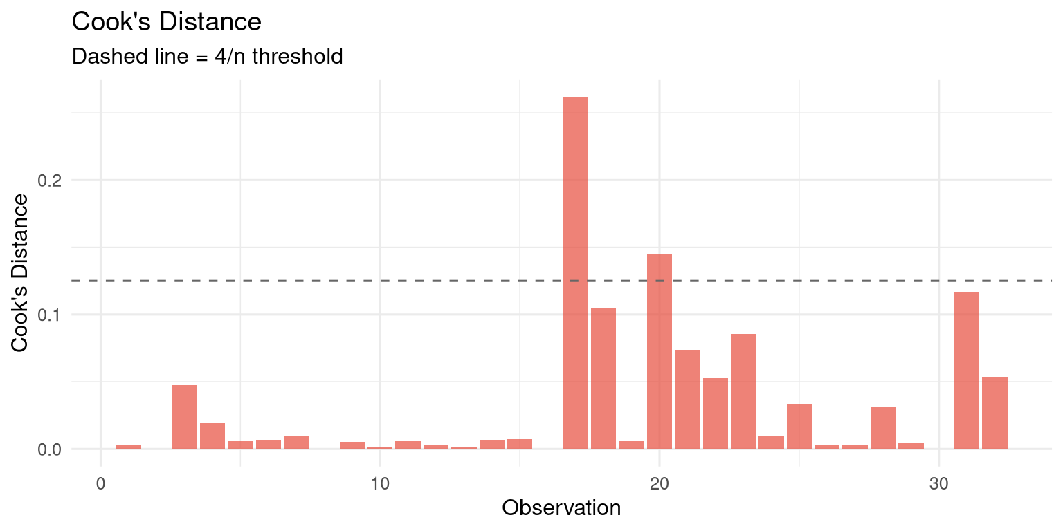
### Influential Observations {#sec-influential}
```{r}
#| label: fig-influential
#| fig-cap: "Cook's distance identifies observations with high influence on the model."
#| fig-width: 8
#| fig-height: 4
augmented |>
mutate(obs = row_number()) |>
ggplot(aes(x = obs, y = .cooksd)) +
geom_col(fill = "#e74c3c", alpha = 0.7) +
geom_hline(yintercept = 4 / nrow(mtcars),
linetype = "dashed", colour = "grey40") +
labs(title = "Cook's Distance",
subtitle = "Dashed line = 4/n threshold",
x = "Observation", y = "Cook's Distance") +
theme_minimal(base_size = 12)
# Which observations have high influence?
augmented |>
arrange(desc(.cooksd)) |>
select(.rownames, mpg, wt, hp, .fitted, .cooksd) |>
head(5)
```
## Using `broom` for Tidy Model Output {#sec-broom}
```{r}
#| label: broom-demo
# Tidy coefficient table
tidy(m_mlr, conf.int = TRUE)
# Model-level statistics
glance(m_mlr)
# Observation-level statistics (fitted, residuals, leverage, etc.)
augment(m_mlr) |> head(5)
```
## Exercises {#sec-ch10-exercises}
1. Using the `mtcars` dataset, regress `qsec` (quarter-mile time) on `hp` and `wt`. Interpret each coefficient and the R-squared value. Are the coefficients statistically significant?
2. Fit three nested regression models predicting `Ozone` in the `airquality` dataset: (a) `Solar.R` only, (b) `Solar.R + Wind`, (c) `Solar.R + Wind + Temp`. Compare them using `anova()` and AIC. Which model is best?
3. Conduct a full diagnostic analysis for model (c) from Exercise 2. Are the assumptions satisfied? If not, what would you do?
4. Add an interaction term to your model: `Wind * Temp`. Is the interaction significant? Interpret what it means.
5. **Challenge:** Download India district-level crop yield data and build a multiple regression model predicting wheat yield from rainfall, fertiliser use, and irrigated area. Present your model in a clean `modelsummary` table and write a brief interpretation of each coefficient.