# Mixed Effects Models {#sec-mixed}
```{r}
#| label: setup-ch12
#| include: false
library(tidyverse)
library(lme4)
library(broom.mixed)
set.seed(42)
```
::: {.callout-note}
## Learning Objectives
By the end of this chapter, you will be able to:
- Explain the difference between fixed and random effects
- Identify situations where mixed models are appropriate
- Fit linear and generalised linear mixed models using `lme4`
- Interpret random intercept and random slope models
- Extract and visualise random effects
:::
## Fixed vs. Random Effects {#sec-fixed-random}
**Fixed effects** are the factors whose specific levels we care about — variety A vs. variety B, urban vs. rural, male vs. female.
**Random effects** are grouping factors where the specific levels are a *sample* from a larger population of possible levels — specific schools, villages, districts, patients, years. We model their *variance* rather than estimating a coefficient for each level.
**Why does this matter?** Standard regression assumes all observations are independent. When observations are nested within groups (students within schools, repeat measures within individuals), this assumption is violated. Mixed models account for this **clustering**.
## When to Use Mixed Models {#sec-when-mixed}
Mixed models are appropriate for:
- **Repeated measures:** Same subject measured multiple times
- **Longitudinal data:** Observations over time within units
- **Nested designs:** Students in classrooms, fields in villages, patients in hospitals
- **Panel data:** Cross-sectional units observed across multiple time periods
## Fitting Mixed Models with `lme4` {#sec-lme4}
### Random Intercept Model {#sec-random-intercept}
```{r}
#| label: mixed-data
# Simulate: crop yield measured in multiple plots within 20 villages, over 5 years
set.seed(123)
n_villages <- 20
n_years <- 5
n_plots <- 8
panel_data <- expand_grid(
village = paste("V", str_pad(1:n_villages, 2, pad = "0"), sep = ""),
year = 2019:2023,
plot = 1:n_plots
) |>
mutate(
village_effect = rep(rnorm(n_villages, 0, 300), each = n_years * n_plots),
rainfall_mm = round(rnorm(n(), 800, 120)),
fertiliser_kg = round(runif(n(), 50, 150)),
yield = 3500 +
0.8 * rainfall_mm +
3.2 * fertiliser_kg +
village_effect +
rnorm(n(), 0, 250)
)
head(panel_data)
```
```{r}
#| label: random-intercept-fit
# Random intercept: each village gets its own intercept
m_ri <- lmer(yield ~ rainfall_mm + fertiliser_kg + (1 | village),
data = panel_data, REML = TRUE)
summary(m_ri)
```
```{r}
#| label: random-intercept-interpret
# Fixed effects
fixef(m_ri)
# Random effects (BLUPs — Best Linear Unbiased Predictors)
ranef(m_ri)$village |> head(8)
# Intraclass Correlation Coefficient
performance::icc(m_ri)
```
The **ICC** tells us what proportion of total variance is due to village-level clustering. A high ICC (> 0.1) justifies a mixed model.
### Random Slope Model {#sec-random-slope}
```{r}
#| label: random-slope-fit
# Random intercept AND slope: fertiliser effect varies by village
m_rs <- lmer(yield ~ rainfall_mm + fertiliser_kg + (1 + fertiliser_kg | village),
data = panel_data, REML = TRUE)
# Compare models
anova(m_ri, m_rs)
```
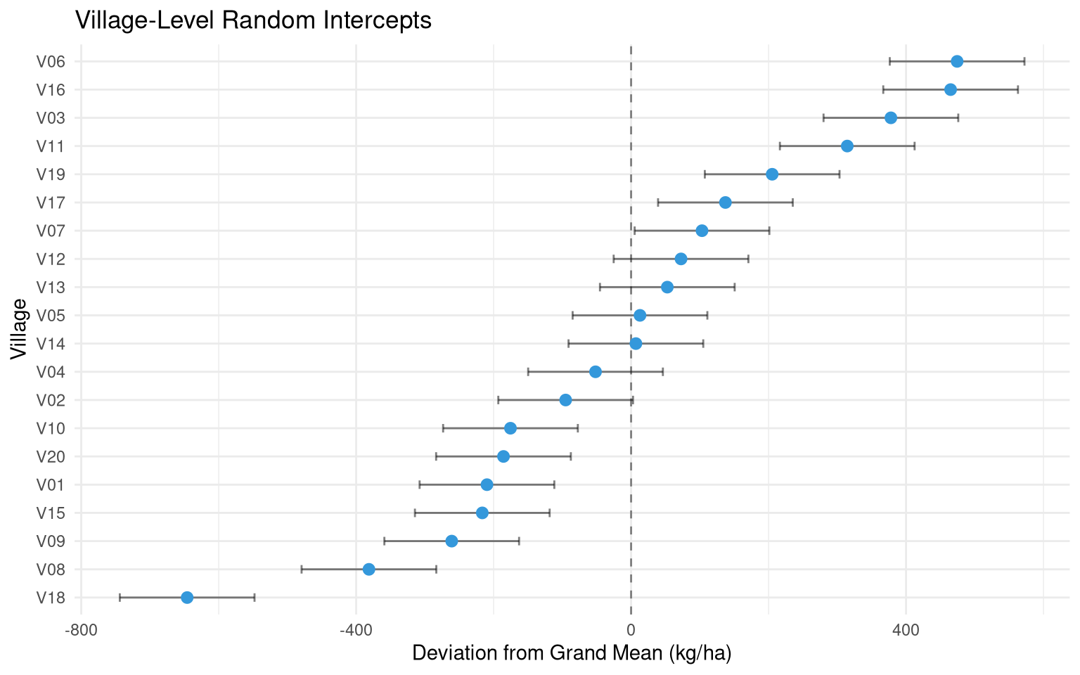
```{r}
#| label: fig-random-effects
#| fig-cap: "Random intercepts for each village — some consistently produce higher yields."
#| fig-width: 8
#| fig-height: 5
ranef_df <- ranef(m_ri)$village |>
  rownames_to_column("village") |>
  rename(intercept = `(Intercept)`) |>
  arrange(intercept)

ggplot(ranef_df, aes(x = intercept, y = reorder(village, intercept))) +
  geom_vline(xintercept = 0, linetype = "dashed", colour = "grey50") +
  geom_errorbarh(aes(xmin = intercept - 1.96 * 50, xmax = intercept + 1.96 * 50),
                 height = 0.3, alpha = 0.5) +
  geom_point(colour = "#3498db", size = 2.5) +
  labs(title = "Village-Level Random Intercepts",
       x = "Deviation from Grand Mean (kg/ha)", y = "Village") +
  theme_minimal(base_size = 11)
```
### Generalised Linear Mixed Models (GLMM) {#sec-glmm}
For binary or count outcomes with clustering:
```{r}
#| label: glmm-fit
# Binary outcome: whether a plot achieved above-median yield
panel_data <- panel_data |>
mutate(high_yield = as.integer(yield > median(yield)))
m_glmm <- glmer(
high_yield ~ rainfall_mm + fertiliser_kg + (1 | village),
data = panel_data,
family = binomial(link = "logit")
)
broom.mixed::tidy(m_glmm, exponentiate = TRUE, conf.int = TRUE) |>
filter(effect == "fixed")
```
## Exercises {#sec-ch12-exercises}
1. Simulate a panel dataset with 15 schools, 30 students per school, and a student-level test score outcome. Fit a random intercept model with student characteristics as fixed effects. Report the ICC.
2. Using the `sleepstudy` dataset from `lme4` (reaction time over days of sleep deprivation), fit a random slope model where the effect of days can vary by subject. Is there significant between-subject variation in the sleep deprivation effect?
3. Compare a standard linear regression (ignoring clustering) with a mixed model on the same data. How do the standard errors differ? What are the implications for inference?