---
title: "Chapter 3: Regression Analysis"
description: "Simple and multiple linear regression, OLS, diagnostics, and interpretation using R."
author: "Pawan Jangra"
date: "2025-02-05"
toc: true
number-sections: true
---
> **Learning Objectives:** Fit and interpret simple and multiple linear regression models, check OLS assumptions through diagnostic plots, and communicate results clearly.
## What is Regression?
Regression analysis quantifies the **relationship between variables**. The goal is to model how changes in **explanatory variables** (X) are associated with changes in the **outcome variable** (Y).
The linear regression model: $Y_i = \beta_0 + \beta_1 X_{1i} + \cdots + \beta_k X_{ki} + \varepsilon_i$
```{r setup}
#| message: false
library(tidyverse)
library(knitr)
library(broom)

# Wage dataset with labour economics flavor
set.seed(2025)
n <- 800
wage_data <- data.frame(
  edu_years = sample(0:20, n, replace=TRUE, prob=dpois(0:20, 9)+0.01),
  experience = sample(0:40, n, replace=TRUE),
  female = rbinom(n, 1, 0.4),
  urban = rbinom(n, 1, 0.55),
  union = rbinom(n, 1, 0.18)
) |>
  mutate(
    log_wage = 4.5 + 0.08*edu_years + 0.04*experience - 0.003*experience^2
               - 0.25*female + 0.15*urban + 0.12*union + rnorm(n, 0, 0.35),
    wage = round(exp(log_wage))
  )
```
## Simple Linear Regression
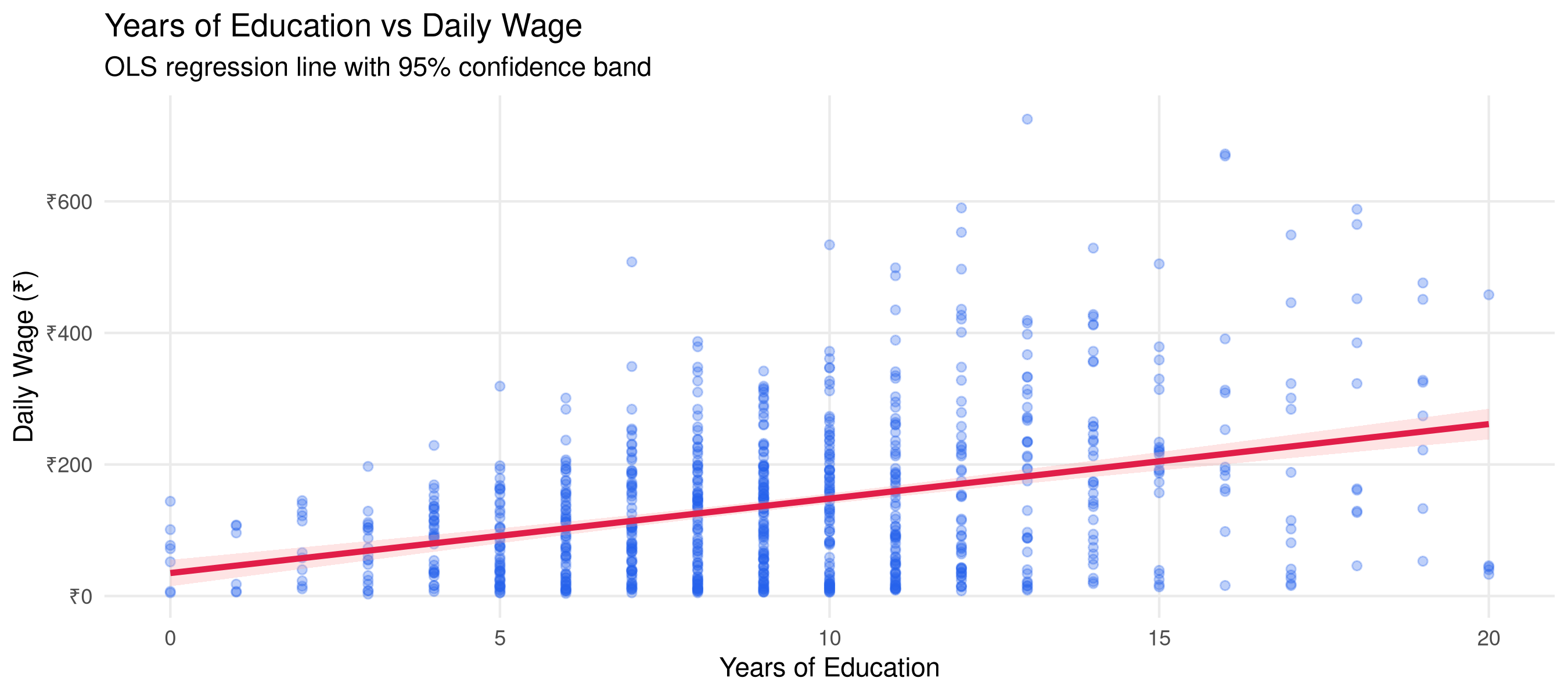
Let's first explore the education-wage relationship:
```{r slr}
#| fig-height: 4
# Scatter with regression line
ggplot(wage_data, aes(x=edu_years, y=wage)) +
  geom_point(alpha=0.3, color="#2563eb", size=1.5) +
  geom_smooth(method="lm", color="#e11d48", se=TRUE, linewidth=1.2,
              fill="#fca5a5", alpha=0.3) +
  scale_y_continuous(labels=scales::label_number(prefix="₹")) +
  labs(title="Years of Education vs Daily Wage",
       subtitle="OLS regression line with 95% confidence band",
       x="Years of Education", y="Daily Wage (₹)") +
  theme_minimal(base_size=11) +
  theme(panel.grid.minor=element_blank())
```
```{r slr-fit}
# Fit simple linear regression
model_simple <- lm(wage ~ edu_years, data=wage_data)
tidy(model_simple) |>
  mutate(across(where(is.numeric), round, 3)) |>
  kable(caption="Simple Linear Regression: Wage ~ Education")
```
```{r slr-r2}
glance(model_simple) |>
  select(r.squared, adj.r.squared, sigma, statistic, p.value, nobs) |>
  mutate(across(where(is.numeric), round, 4)) |>
  kable(caption="Model fit statistics")
```
**Interpretation:** For each additional year of education, daily wages increase by ₹`r round(coef(model_simple)[2])` on average, holding all else constant.
## Multiple Linear Regression
Now let's add more variables:
```{r mlr}
model_full <- lm(wage ~ edu_years + experience + I(experience^2) +
                   female + urban + union, data=wage_data)

tidy(model_full) |>
  mutate(
    term = recode(term,
      `(Intercept)`="Intercept",
      edu_years="Education (years)",
      experience="Experience (years)",
      `I(experience^2)`="Experience² (quadratic)",
      female="Female (=1)",
      urban="Urban (=1)",
      union="Union member (=1)"
    ),
    across(where(is.numeric), round, 4),
    significance = case_when(
      p.value < 0.001 ~ "***",
      p.value < 0.01  ~ "**",
      p.value < 0.05  ~ "*",
      TRUE            ~ ""
    )
  ) |>
  kable(caption="Multiple Regression Results (*** p<0.001, ** p<0.01, * p<0.05)")
```
```{r model-comparison}
# Compare models
bind_rows(
  glance(model_simple) |> mutate(Model="Simple (Education only)"),
  glance(model_full)   |> mutate(Model="Full Model")
) |>
  select(Model, r.squared, adj.r.squared, sigma, AIC) |>
  mutate(across(where(is.numeric), round, 3)) |>
  kable(caption="Model comparison")
```
## Regression Diagnostics
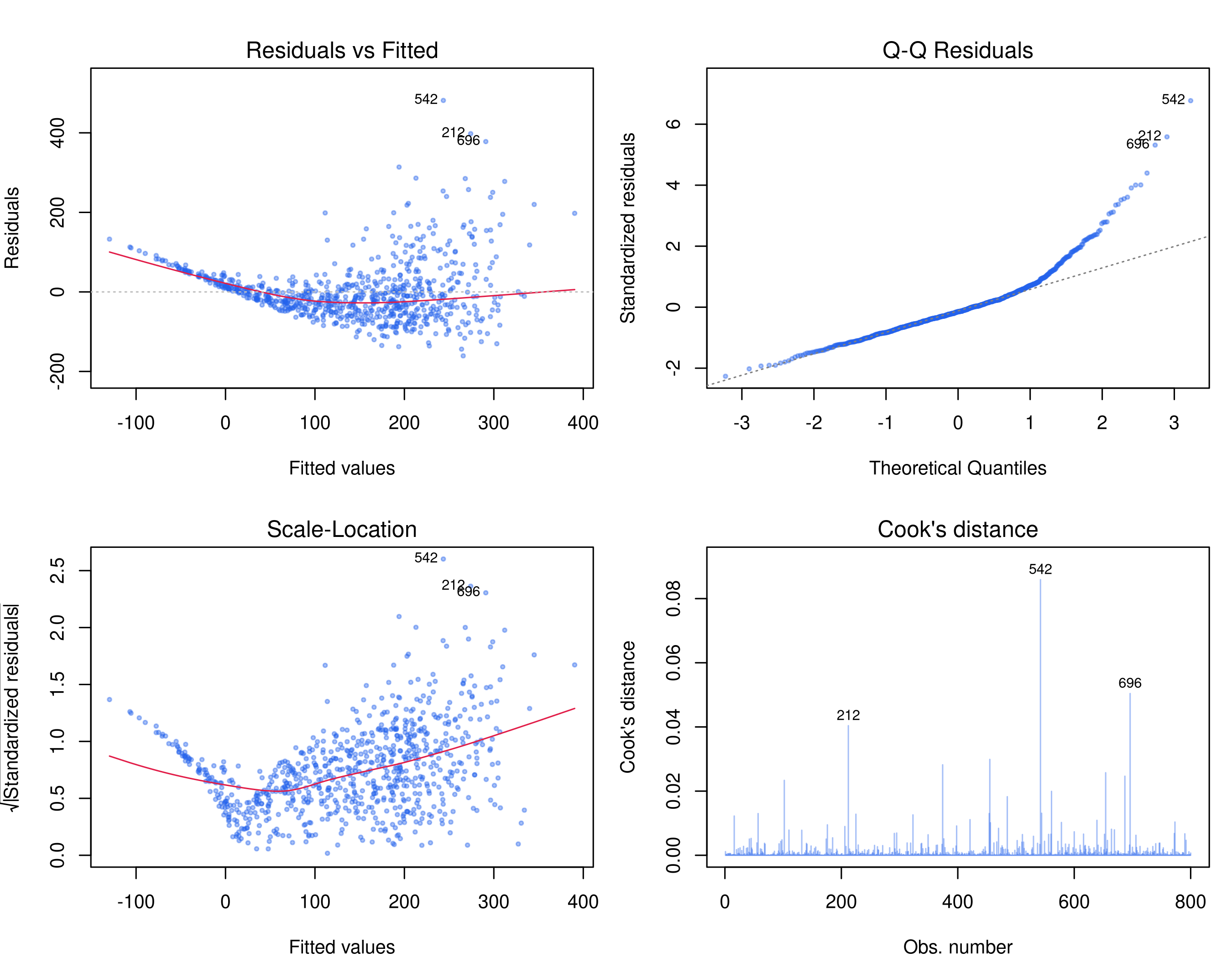
Always check the four core OLS assumptions:
```{r diagnostics}
#| fig-height: 7
#| fig-cap: "Regression diagnostic plots — checking OLS assumptions"
par(mfrow=c(2,2), mar=c(4,4,3,1), family="sans")
plot(model_full, which=1:4,
     col=alpha("#2563eb", 0.4), pch=20, cex=0.7,
     col.smooth="#e11d48", lwd.smooth=2)
par(mfrow=c(1,1))
```
**What to look for:**
- **Residuals vs Fitted:** Should show no pattern (random scatter around 0)
- **Q-Q Plot:** Points should follow the diagonal line (normality of residuals)
- **Scale-Location:** Horizontal band (homoscedasticity — equal variance)
- **Cook's Distance:** Points above 0.5 are influential observations
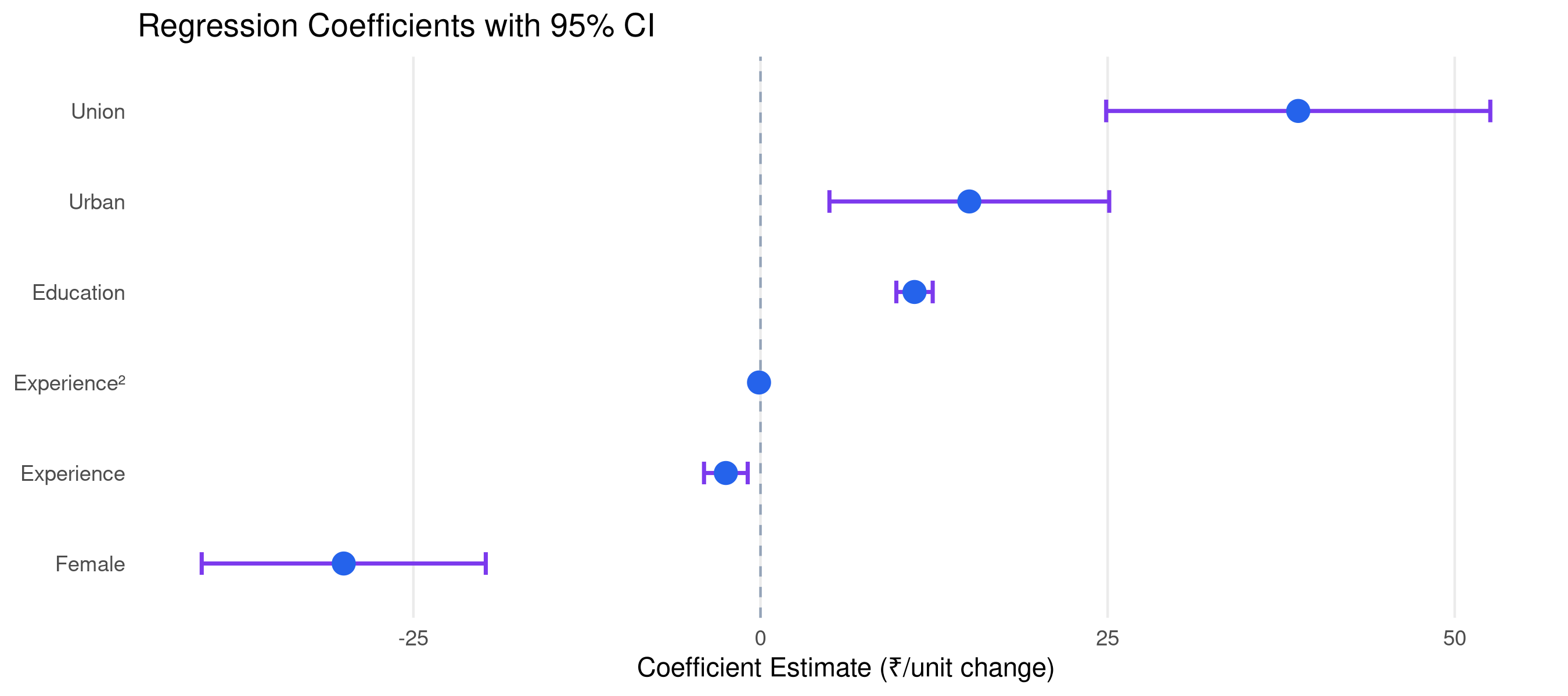
## Coefficient Plot
```{r coef-plot}
#| fig-height: 4
tidy(model_full, conf.int=TRUE) |>
  filter(term != "(Intercept)") |>
  mutate(term = recode(term,
    edu_years="Education", experience="Experience",
    `I(experience^2)`="Experience²",
    female="Female", urban="Urban", union="Union")) |>
  ggplot(aes(x=estimate, y=reorder(term, estimate))) +
  geom_vline(xintercept=0, linetype="dashed", color="#94a3b8") +
  geom_errorbarh(aes(xmin=conf.low, xmax=conf.high), height=0.25,
                 color="#7c3aed", linewidth=0.8) +
  geom_point(size=4, color="#2563eb") +
  labs(title="Regression Coefficients with 95% CI",
       x="Coefficient Estimate (₹/unit change)", y=NULL) +
  theme_minimal(base_size=11) +
  theme(panel.grid.minor=element_blank(),
        panel.grid.major.y=element_blank())
```
## Log-Linear Wage Equation (Mincer Model)
A standard approach in labour economics — using log wages gives percentage interpretations:
```{r mincer}
model_log <- lm(log_wage ~ edu_years + experience + I(experience^2) +
                  female + urban + union, data=wage_data)

tidy(model_log) |>
  filter(term != "(Intercept)") |>
  mutate(
    term = recode(term,
      edu_years="Education (years)",
      experience="Experience",
      `I(experience^2)`="Experience²",
      female="Female (=1)",
      urban="Urban (=1)",
      union="Union (=1)"),
    pct_effect = round((exp(estimate)-1)*100, 2),
    across(c(estimate, std.error, p.value), round, 4)
  ) |>
  select(term, estimate, std.error, p.value, pct_effect) |>
  rename(`% Effect` = pct_effect) |>
  kable(caption="Mincer Wage Equation (Log-Linear): % change in wage per unit")
```
**Key finding:** The gender wage gap is approximately `r round((1 - exp(coef(model_log)["female"]))*100, 1)`% — women earn about this much less than men after controlling for education, experience, and other factors.
## Practice Exercises
::: {.callout-tip}
## Try It Yourself
1. Add state fixed effects to the model using `lm(wage ~ ... + factor(state))`
2. Test for heteroscedasticity using `lmtest::bptest()`
3. Compute robust standard errors using `sandwich::vcovHC()`
4. Interpret the experience² coefficient — at what experience level do wages peak?
:::
**Next:** [Chapter 4 — Time Series Analysis →](chapter4.html)