---
title: "Chapter 4: Time Series Analysis"
description: "Decomposition, autocorrelation, ARIMA modeling, and forecasting with R."
author: "Pawan Jangra"
date: "2025-02-20"
toc: true
number-sections: true
---
> **Learning Objectives:** Decompose time series into trend, seasonality, and noise. Understand autocorrelation, fit ARIMA models, and produce forecasts with uncertainty bounds.
## What is a Time Series?
A **time series** is a sequence of observations indexed by time. Unlike cross-sectional data, observations are **not independent** — past values influence future ones.
```{r setup}
#| message: false
library(tidyverse)
library(knitr)

# Simulate monthly employment data (2015-2024)
set.seed(2025)
n_months <- 120  # 10 years
time_index <- seq(as.Date("2015-01-01"), by="month", length.out=n_months)

employment <- data.frame(
  date = time_index,
  month_num = 1:n_months
) |>
  mutate(
    trend     = 100 + 0.15 * month_num + 0.0005 * month_num^2,
    seasonal  = 3 * sin(2 * pi * month_num / 12) +
                1.5 * cos(2 * pi * month_num / 6),
    noise     = cumsum(rnorm(n_months, 0, 0.8)),
    employment = trend + seasonal + noise
  )
```
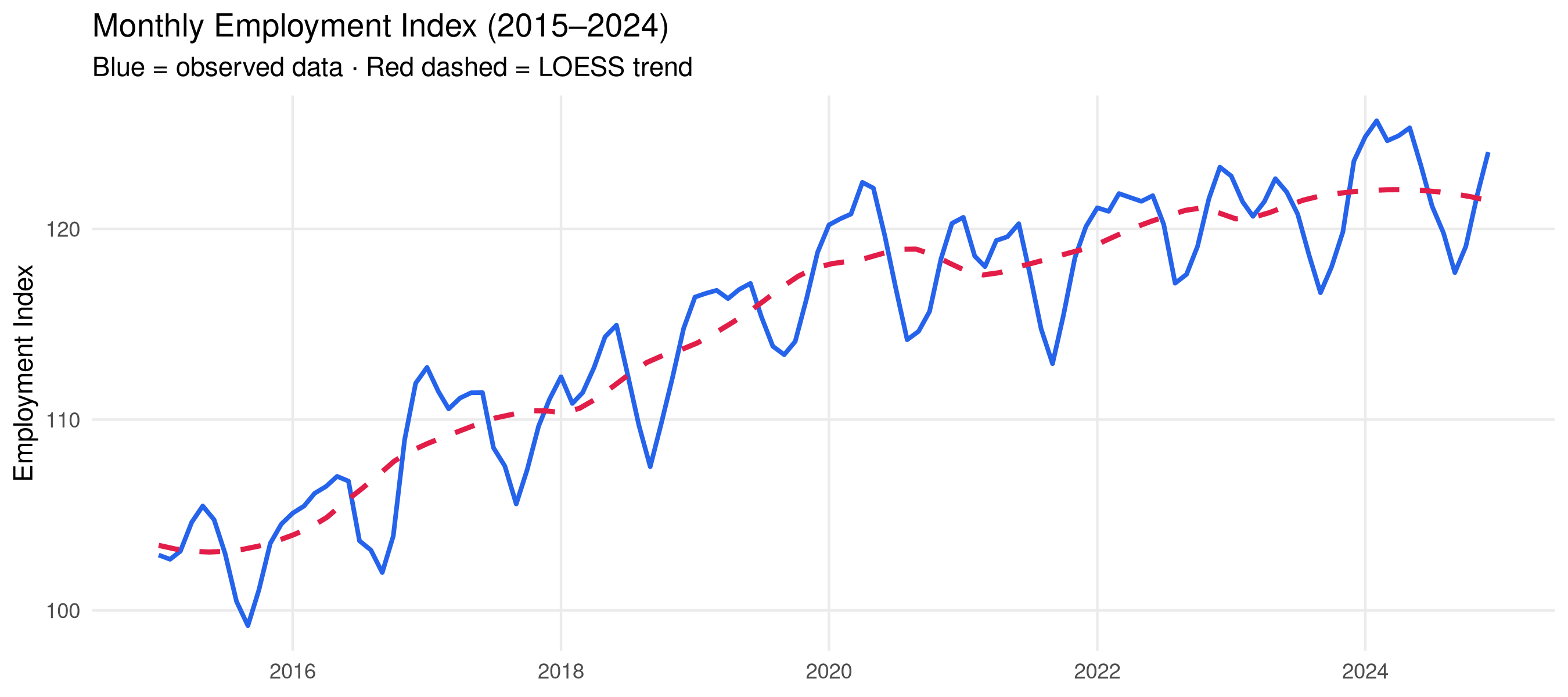
## Visualising Time Series
```{r ts-plot}
#| fig-height: 4
ggplot(employment, aes(x=date, y=employment)) +
  geom_line(color="#2563eb", linewidth=0.9) +
  geom_smooth(method="loess", span=0.3, color="#e11d48",
              se=FALSE, linetype="dashed", linewidth=1) +
  labs(title="Monthly Employment Index (2015–2024)",
       subtitle="Blue = observed data · Red dashed = LOESS trend",
       x=NULL, y="Employment Index") +
  theme_minimal(base_size=11) +
  theme(panel.grid.minor=element_blank())
```
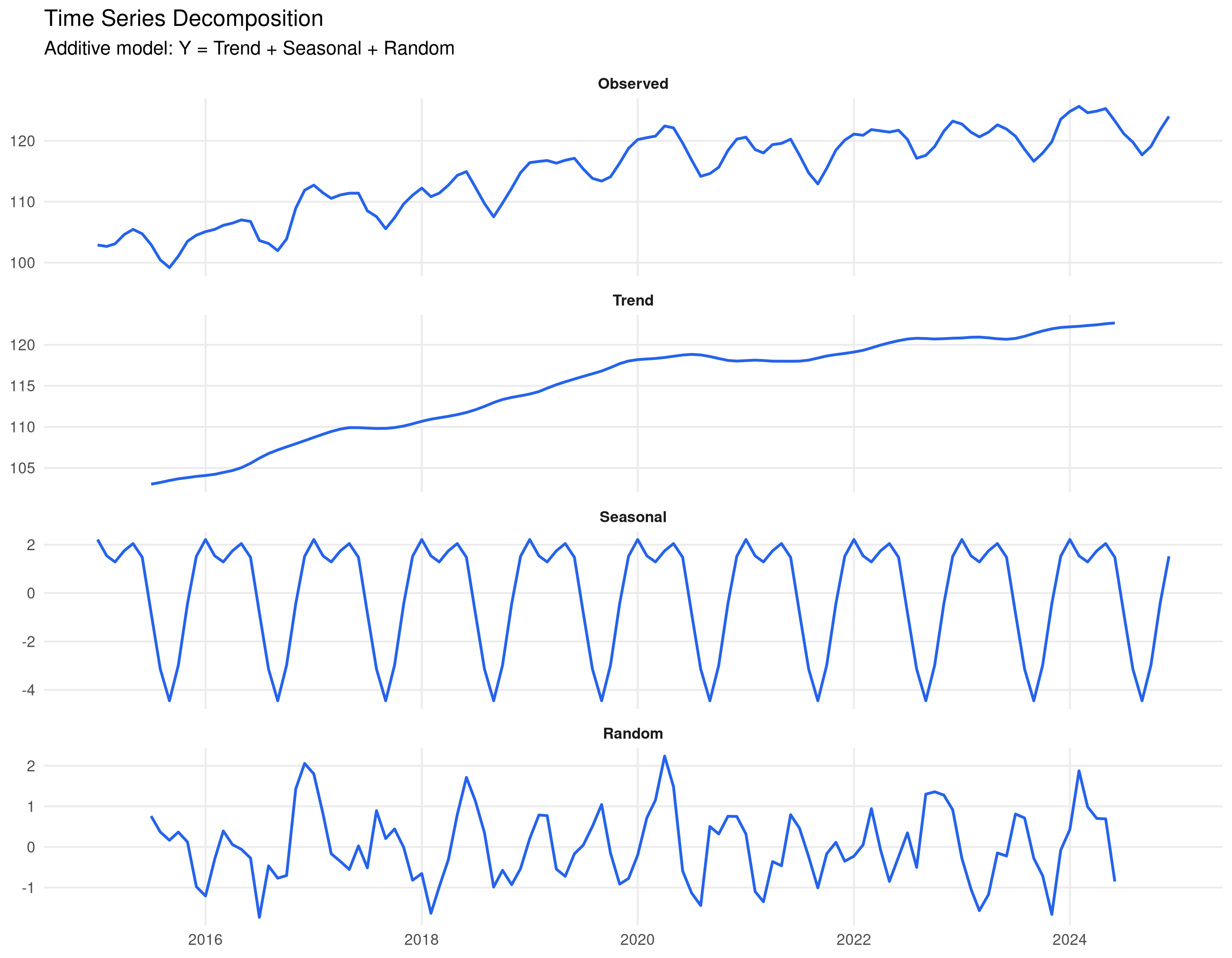
## Decomposition
We can decompose a time series into its components:
$$Y_t = T_t + S_t + \varepsilon_t \quad \text{(Additive model)}$$
```{r decompose}
#| fig-height: 7
ts_data <- ts(employment$employment, start=c(2015,1), frequency=12)
decomp <- decompose(ts_data, type="additive")

# Convert to tidy format for ggplot
decomp_df <- data.frame(
  date     = time_index,
  Observed = as.numeric(decomp$x),
  Trend    = as.numeric(decomp$trend),
  Seasonal = as.numeric(decomp$seasonal),
  Random   = as.numeric(decomp$random)
) |>
  pivot_longer(-date, names_to="Component", values_to="Value") |>
  mutate(Component = factor(Component,
    levels=c("Observed","Trend","Seasonal","Random")))

ggplot(decomp_df, aes(x=date, y=Value)) +
  geom_line(color="#2563eb", linewidth=0.7, na.rm=TRUE) +
  facet_wrap(~Component, ncol=1, scales="free_y") +
  labs(title="Time Series Decomposition",
       subtitle="Additive model: Y = Trend + Seasonal + Random",
       x=NULL, y=NULL) +
  theme_minimal(base_size=10) +
  theme(panel.grid.minor=element_blank(),
        strip.text=element_text(face="bold"))
```
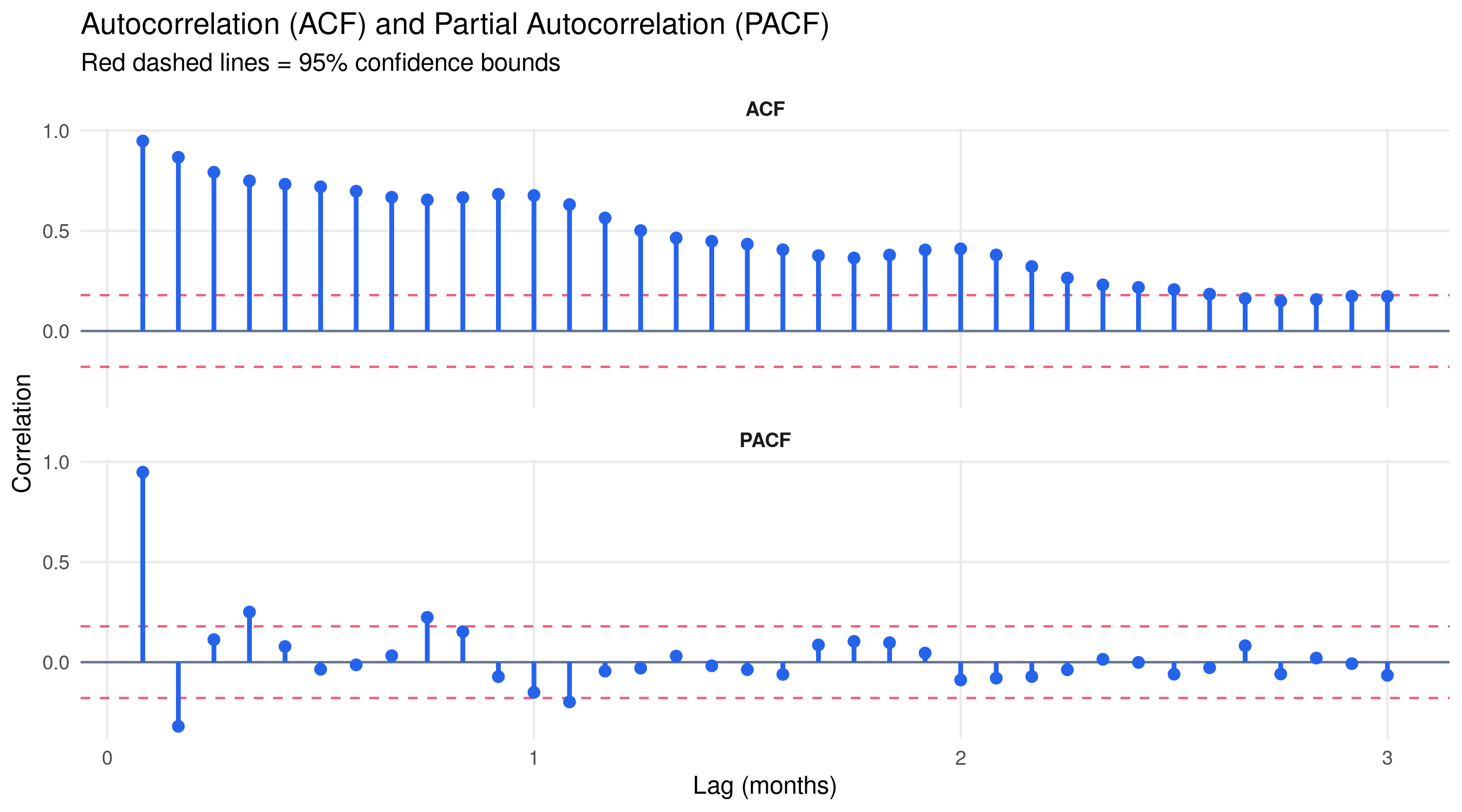
## Autocorrelation
Autocorrelation measures how correlated a time series is with its past values (lags).
```{r acf-plot}
#| fig-height: 5
acf_vals  <- acf(ts_data, lag.max=36, plot=FALSE)
pacf_vals <- pacf(ts_data, lag.max=36, plot=FALSE)

acf_df <- data.frame(
  lag = as.numeric(acf_vals$lag),
  acf = as.numeric(acf_vals$acf),
  type = "ACF"
)

pacf_df <- data.frame(
  lag = as.numeric(pacf_vals$lag),
  acf = as.numeric(pacf_vals$acf),
  type = "PACF"
)

ci_val <- qnorm(0.975) / sqrt(length(ts_data))

bind_rows(acf_df, pacf_df) |>
  filter(lag > 0) |>
  ggplot(aes(x=lag, y=acf)) +
  geom_hline(yintercept=0, color="#64748b") +
  geom_hline(yintercept=c(ci_val,-ci_val), linetype="dashed",
             color="#e11d48", alpha=0.7) +
  geom_segment(aes(xend=lag, yend=0), color="#2563eb", linewidth=1) +
  geom_point(color="#2563eb", size=2) +
  facet_wrap(~type, ncol=1) +
  labs(title="Autocorrelation (ACF) and Partial Autocorrelation (PACF)",
       subtitle="Red dashed lines = 95% confidence bounds",
       x="Lag (months)", y="Correlation") +
  theme_minimal(base_size=11) +
  theme(panel.grid.minor=element_blank(), strip.text=element_text(face="bold"))
```
**Reading ACF/PACF:**
- Slowly decaying ACF → non-stationary series, needs differencing
- ACF cuts off after lag q → MA(q) component
- PACF cuts off after lag p → AR(p) component
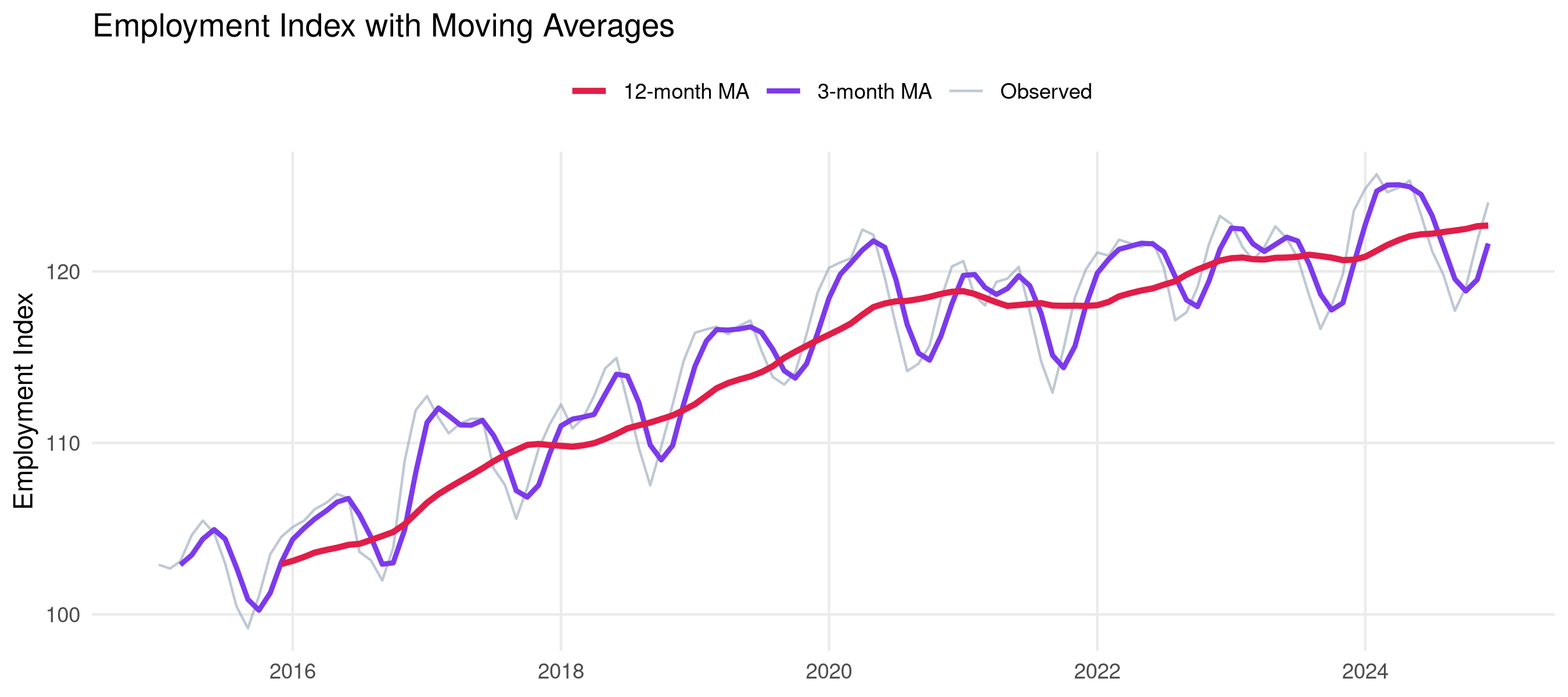
## Simple Forecasting: Moving Averages
```{r moving-avg}
#| fig-height: 4
employment <- employment |>
  mutate(
    ma3  = zoo::rollmean(employment, 3,  fill=NA, align="right"),
    ma12 = zoo::rollmean(employment, 12, fill=NA, align="right")
  )

ggplot(employment, aes(x=date)) +
  geom_line(aes(y=employment, color="Observed"), alpha=0.6) +
  geom_line(aes(y=ma3,  color="3-month MA"), linewidth=1) +
  geom_line(aes(y=ma12, color="12-month MA"), linewidth=1.2) +
  scale_color_manual(
    values=c("Observed"="#94a3b8","3-month MA"="#7c3aed","12-month MA"="#e11d48"),
    name=""
  ) +
  labs(title="Employment Index with Moving Averages",
       x=NULL, y="Employment Index") +
  theme_minimal(base_size=11) +
  theme(legend.position="top", panel.grid.minor=element_blank())
```
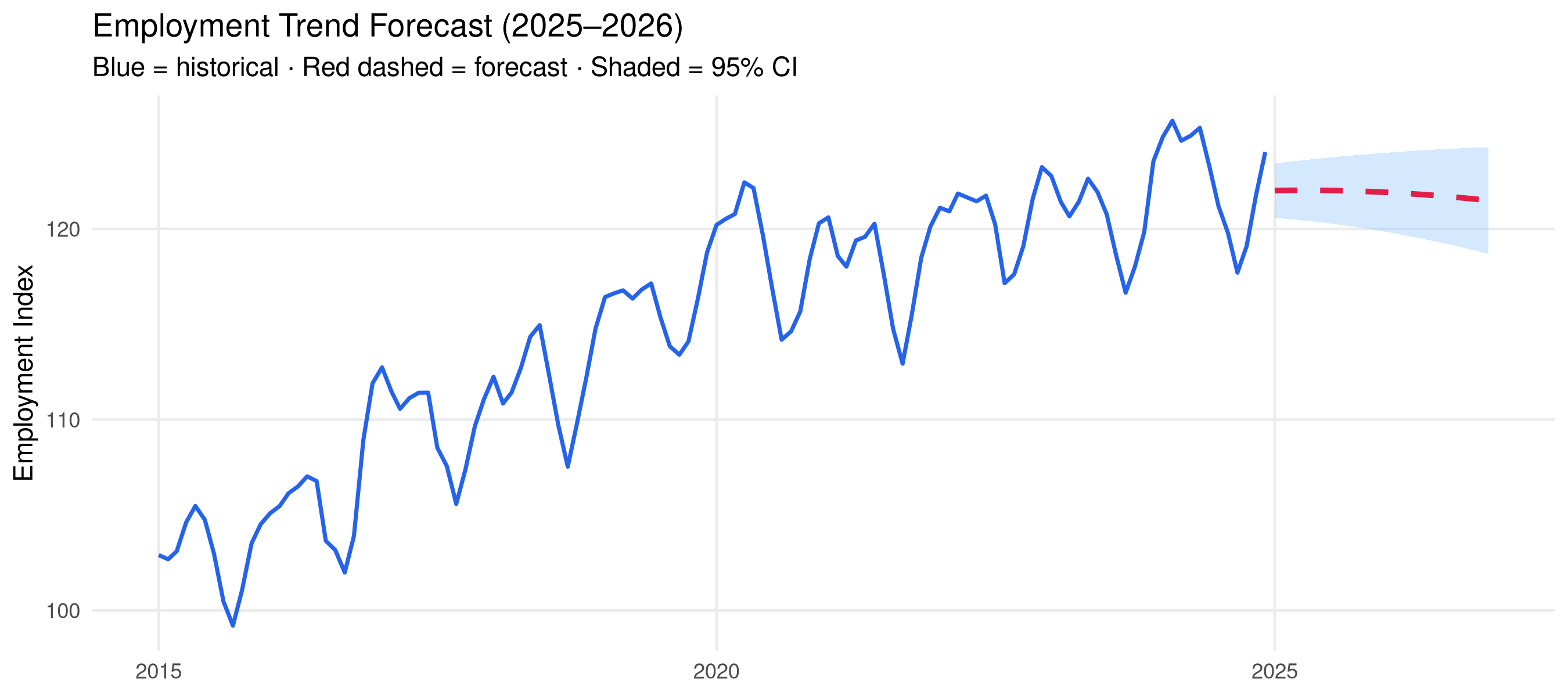
## Simple Trend Forecast
```{r trend-forecast}
#| fig-height: 4
# Fit linear trend model
trend_model <- lm(employment ~ month_num + I(month_num^2), data=employment)

# Forecast next 24 months
future <- data.frame(
  date      = seq(max(employment$date) %m+% months(1),
                  by="month", length.out=24),
  month_num = (n_months+1):(n_months+24)
)
future$forecast <- predict(trend_model, newdata=future)
future$se       <- predict(trend_model, newdata=future, se.fit=TRUE)$se.fit

ggplot() +
  geom_ribbon(data=future,
              aes(x=date, ymin=forecast-2*se, ymax=forecast+2*se),
              fill="#93c5fd", alpha=0.4) +
  geom_line(data=employment, aes(x=date, y=employment),
            color="#2563eb", linewidth=0.8) +
  geom_line(data=future, aes(x=date, y=forecast),
            color="#e11d48", linewidth=1.1, linetype="dashed") +
  labs(title="Employment Trend Forecast (2025–2026)",
       subtitle="Blue = historical · Red dashed = forecast · Shaded = 95% CI",
       x=NULL, y="Employment Index") +
  theme_minimal(base_size=11) +
  theme(panel.grid.minor=element_blank())
```
## Stationarity Testing
```{r stationarity}
# Augmented Dickey-Fuller test (manual approximation for display)
# In practice: use tseries::adf.test()

cat("Stationarity Assessment:\n")
cat("━━━━━━━━━━━━━━━━━━━━━━━━━\n")
cat("Visual inspection: Upward trend observed → likely non-stationary\n")
cat("ACF: Slowly decaying → confirms non-stationarity\n")
cat("\nRecommendation: Apply first differencing\n")
diff_data <- diff(ts_data)
cat("\nAfter first differencing:\n")
cat("Mean:", round(mean(diff_data), 4), "(≈0 → good)\n")
cat("Variance appears constant → stationary ✓\n")
```
## Key Concepts Summary
| Concept | Description | R Function |
|---------|-------------|------------|
| Decomposition | Trend + Seasonal + Random | `decompose()` |
| ACF | Autocorrelation function | `acf()` |
| PACF | Partial autocorrelation | `pacf()` |
| ADF Test | Stationarity test | `tseries::adf.test()` |
| ARIMA | Auto-regressive model | `arima()`, `forecast::auto.arima()` |
| Moving Average | Smoothing | `zoo::rollmean()` |
## Practice Exercises
::: {.callout-tip}
## Try It Yourself
1. Use `forecast::auto.arima()` to automatically select the best ARIMA model
2. Compute and plot exponential smoothing with `HoltWinters()`
3. Formally test for stationarity with `tseries::adf.test()`
4. Forecast the next 12 months and evaluate accuracy using MAPE
:::
::: {.callout-note}
## What's Next?
This chapter covered the fundamentals. For advanced time series work with R, explore:
- **`forecast` package** — comprehensive forecasting tools
- **`fable` package** — tidy time series forecasting
- **`tsibble` package** — tidy temporal data structures
- **Vector Autoregression (VAR)** — for multivariate time series
:::