Chapter 1: Descriptive Statistics

Measures of central tendency, dispersion, shape, and exploratory data analysis with R.

Author

Pawan Jangra

Published

January 10, 2025

Learning Objectives: By the end of this chapter, you will be able to compute and interpret measures of central tendency and dispersion, create effective visualizations for exploring distributions, and identify skewness and outliers in real datasets.

1 Introduction to Descriptive Statistics

Descriptive statistics summarize and describe the main features of a dataset. They are the first step in any data analysis — before we run a single regression or hypothesis test, we must understand what our data looks like.

In R, we have powerful tools for this. Let’s load our packages and create a realistic dataset:

library(tidyverse)
library(knitr)

# Simulate Labour Force Survey data
set.seed(2025)
n <- 1000

lfs_data <- data.frame(
  age       = round(rnorm(n, 35, 12)) |> pmax(15) |> pmin(70),
  wage      = exp(rnorm(n, log(400), 0.7)) |> round(),
  edu_years = sample(0:20, n, replace = TRUE, 
                     prob = dpois(0:20, 8) + 0.01),
  gender    = sample(c("Male","Female"), n, replace = TRUE, prob=c(.6,.4)),
  state     = sample(c("Haryana","UP","Bihar","Maharashtra","Karnataka"), 
                     n, replace = TRUE),
  sector    = sample(c("Agriculture","Industry","Services"), n, 
                     replace = TRUE, prob = c(.4,.2,.4))
)

glimpse(lfs_data)

Rows: 1,000
Columns: 6
$ age       <dbl> 42, 35, 44, 50, 39, 33, 40, 34, 31, 43, 30, 15, 30, 44, 48, …
$ wage      <dbl> 737, 93, 261, 148, 239, 242, 229, 505, 385, 337, 256, 148, 2…
$ edu_years <int> 2, 4, 4, 2, 9, 8, 16, 11, 5, 4, 7, 10, 4, 9, 10, 6, 10, 13, …
$ gender    <chr> "Male", "Female", "Female", "Female", "Male", "Male", "Femal…
$ state     <chr> "UP", "Maharashtra", "Haryana", "UP", "Karnataka", "Bihar", …
$ sector    <chr> "Services", "Agriculture", "Services", "Industry", "Industry…

2 Measures of Central Tendency

The three main measures of central tendency each tell a different story:

wage_stats <- lfs_data |>
  summarise(
    Mean   = mean(wage),
    Median = median(wage),
    Mode   = as.numeric(names(sort(table(round(wage,-2)), decreasing=TRUE)[1])),
    SD     = sd(wage),
    IQR    = IQR(wage),
    Min    = min(wage),
    Max    = max(wage),
    Skewness = (mean(wage) - median(wage)) / sd(wage) * 3  # Pearson's approx
  ) |>
  pivot_longer(everything(), names_to = "Statistic", values_to = "Value") |>
  mutate(Value = round(Value, 2))

kable(wage_stats, caption = "Descriptive Statistics for Daily Wage (₹)")

Descriptive Statistics for Daily Wage (₹)
Statistic	Value
Mean	505.76
Median	394.00
Mode	200.00
SD	444.35
IQR	397.25
Min	46.00
Max	6001.00
Skewness	0.75

2.1 Why the Mean ≠ Median for Wages

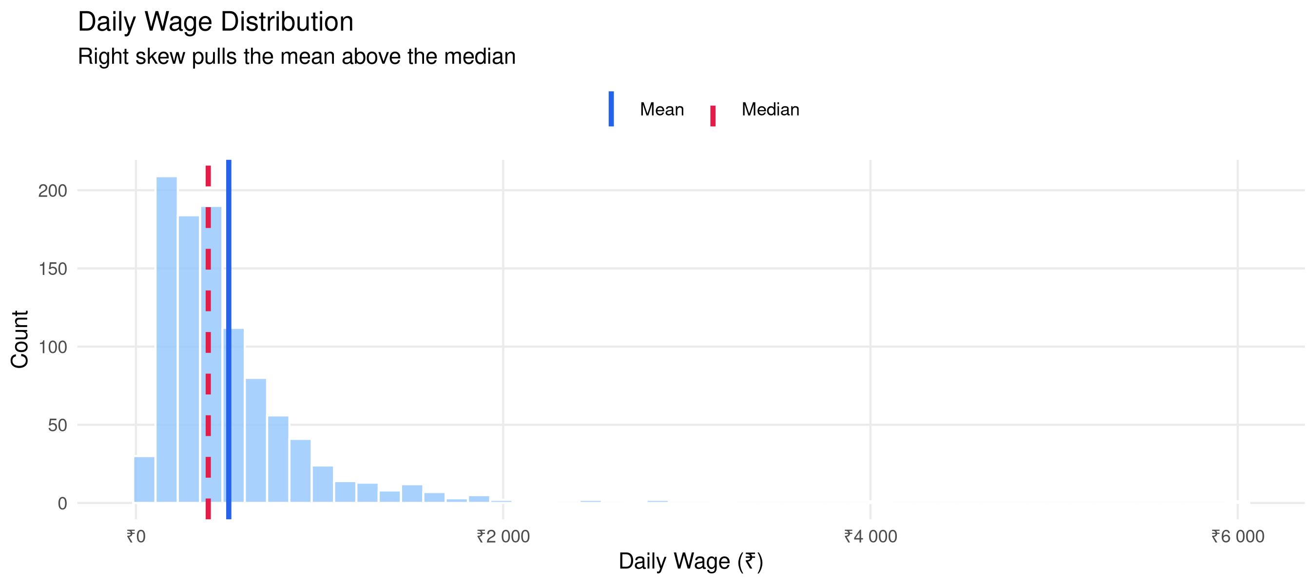
ggplot(lfs_data, aes(x = wage)) +
  geom_histogram(bins = 50, fill = "#93c5fd", alpha = 0.8, color = "white") +
  geom_vline(aes(xintercept = mean(wage), linetype = "Mean"), 
             color = "#2563eb", linewidth = 1.2) +
  geom_vline(aes(xintercept = median(wage), linetype = "Median"), 
             color = "#e11d48", linewidth = 1.2) +
  scale_linetype_manual(name = "", values = c("Mean"="solid","Median"="dashed")) +
  scale_x_continuous(labels = scales::label_number(prefix = "₹")) +
  labs(title = "Daily Wage Distribution",
       subtitle = "Right skew pulls the mean above the median",
       x = "Daily Wage (₹)", y = "Count") +
  theme_minimal(base_size = 11) +
  theme(legend.position = "top", panel.grid.minor = element_blank())

Wage distribution showing mean vs median divergence due to right skew

Key insight: For right-skewed income distributions, the median is almost always a better measure of “typical” than the mean. A few high earners inflate the mean.

3 Measures of Dispersion

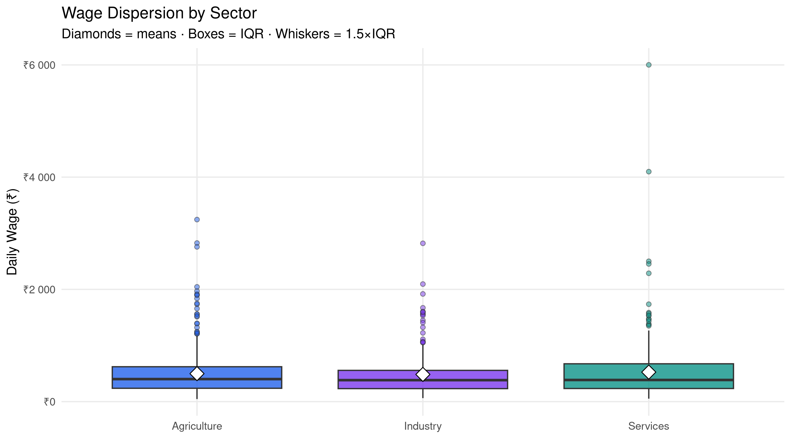
# Boxplot comparison across sectors
ggplot(lfs_data, aes(x = sector, y = wage, fill = sector)) +
  geom_boxplot(alpha = 0.8, outlier.shape = 21, outlier.alpha = 0.5,
               outlier.size = 1.5) +
  stat_summary(fun = mean, geom = "point", shape = 23, 
               size = 4, fill = "white", color = "black") +
  scale_fill_manual(values = c("#2563eb","#7c3aed","#0d9488")) +
  scale_y_continuous(labels = scales::label_number(prefix = "₹")) +
  labs(title = "Wage Dispersion by Sector",
       subtitle = "Diamonds = means · Boxes = IQR · Whiskers = 1.5×IQR",
       x = NULL, y = "Daily Wage (₹)") +
  theme_minimal(base_size = 11) +
  theme(legend.position = "none", panel.grid.minor = element_blank())

dispersion_by_sector <- lfs_data |>
  group_by(sector) |>
  summarise(
    n      = n(),
    Mean   = round(mean(wage)),
    SD     = round(sd(wage)),
    `CV (%)` = round(sd(wage)/mean(wage)*100, 1),
    Median = round(median(wage)),
    IQR    = round(IQR(wage)),
    .groups = "drop"
  )

kable(dispersion_by_sector, 
      caption = "Dispersion measures by sector (CV = Coefficient of Variation)")

Dispersion measures by sector (CV = Coefficient of Variation)
sector	n	Mean	SD	CV (%)	Median	IQR
Agriculture	423	499	406	81.4	402	384
Industry	214	485	400	82.3	383	326
Services	363	526	508	96.6	386	440

Coefficient of Variation (CV): Useful for comparing dispersion across groups with different means. CV = (SD / Mean) × 100%. Higher CV means more relative spread.

4 Exploring Distributions

4.1 Five-Number Summary

five_num <- lfs_data |>
  group_by(gender) |>
  summarise(
    Min    = min(wage),
    Q1     = quantile(wage, 0.25),
    Median = median(wage),
    Q3     = quantile(wage, 0.75),
    Max    = max(wage),
    .groups = "drop"
  )

kable(five_num, digits = 0, 
      caption = "Five-number summary by gender (₹)")

Five-number summary by gender (₹)
gender	Min	Q1	Median	Q3	Max
Female	53	225	395	577	6001
Male	46	241	391	667	4098

4.2 Detecting Outliers

# IQR method for outlier detection
wage_bounds <- lfs_data |>
  summarise(
    Q1  = quantile(wage, 0.25),
    Q3  = quantile(wage, 0.75),
    IQR = IQR(wage),
    lower = Q1 - 1.5 * IQR,
    upper = Q3 + 1.5 * IQR
  )

lfs_outliers <- lfs_data |>
  mutate(is_outlier = wage < wage_bounds$lower | wage > wage_bounds$upper)

cat("Outliers detected (IQR method):", sum(lfs_outliers$is_outlier), "\n")

Outliers detected (IQR method): 54

cat("That's", round(mean(lfs_outliers$is_outlier)*100, 1), "% of observations\n")

That's 5.4 % of observations

5 Cross-tabulation: Two-Way Frequencies

# Sector by state distribution
cross_tab <- lfs_data |>
  count(sector, gender) |>
  pivot_wider(names_from = gender, values_from = n) |>
  mutate(Total = Male + Female,
         `Female Share (%)` = round(Female/Total*100, 1))

kable(cross_tab, caption = "Employment distribution by sector and gender")

Employment distribution by sector and gender
sector	Female	Male	Total	Female Share (%)
Agriculture	189	234	423	44.7
Industry	94	120	214	43.9
Services	143	220	363	39.4

6 Practice Exercises

Try It Yourself

Compute the Gini coefficient for wage inequality using ineq package
Create a violin plot comparing wages across all 5 states
Test whether mean wages differ significantly between sectors using ANOVA
Compute the 90th percentile wage separately for male and female workers

7 Chapter Summary

Concept	Measure	R Function
Central Tendency	Mean	`mean()`
Central Tendency	Median	`median()`
Dispersion	Standard Deviation	`sd()`
Dispersion	IQR	`IQR()`
Shape	Skewness	`moments::skewness()`
Range	Min/Max	`min()`, `max()`
Quantiles	Quartiles	`quantile()`

Next: Chapter 2 — Probability & Distributions →