Code
library(tidyverse)
library(knitr)Learning Objectives: Understand core probability concepts, work with common distributions (Normal, Binomial, Poisson, t), and apply these in real-world contexts using R’s built-in distribution functions.
Every distribution in R has four functions:
| Prefix | Function | Returns |
|---|---|---|
d |
dnorm(x) |
Probability density at x |
p |
pnorm(q) |
P(X ≤ q) — CDF |
q |
qnorm(p) |
Quantile (inverse CDF) |
r |
rnorm(n) |
n random samples |
library(tidyverse)
library(knitr)The Normal distribution is the cornerstone of statistical inference — thanks to the Central Limit Theorem.
# Compare Normal distributions with different parameters
x_vals <- seq(-5, 15, length.out = 500)

normal_df <- bind_rows(
  data.frame(x=x_vals, density=dnorm(x_vals, mean=0, sd=1),   label="N(0,1)"),
  data.frame(x=x_vals, density=dnorm(x_vals, mean=3, sd=1.5), label="N(3,1.5)"),
  data.frame(x=x_vals, density=dnorm(x_vals, mean=5, sd=0.5), label="N(5,0.5)"),
  data.frame(x=x_vals, density=dnorm(x_vals, mean=2, sd=2.5), label="N(2,2.5)")
)

ggplot(normal_df, aes(x=x, y=density, color=label)) +
  geom_line(linewidth=1.2) +
  scale_color_manual(values=c("#2563eb","#7c3aed","#0d9488","#d97706")) +
  labs(title="Normal Distributions with Different Parameters",
       subtitle="Location (μ) shifts the center; Scale (σ) controls spread",
       x="x", y="Density", color="Distribution") +
  theme_minimal(base_size=11) +
  theme(legend.position="right", panel.grid.minor=element_blank())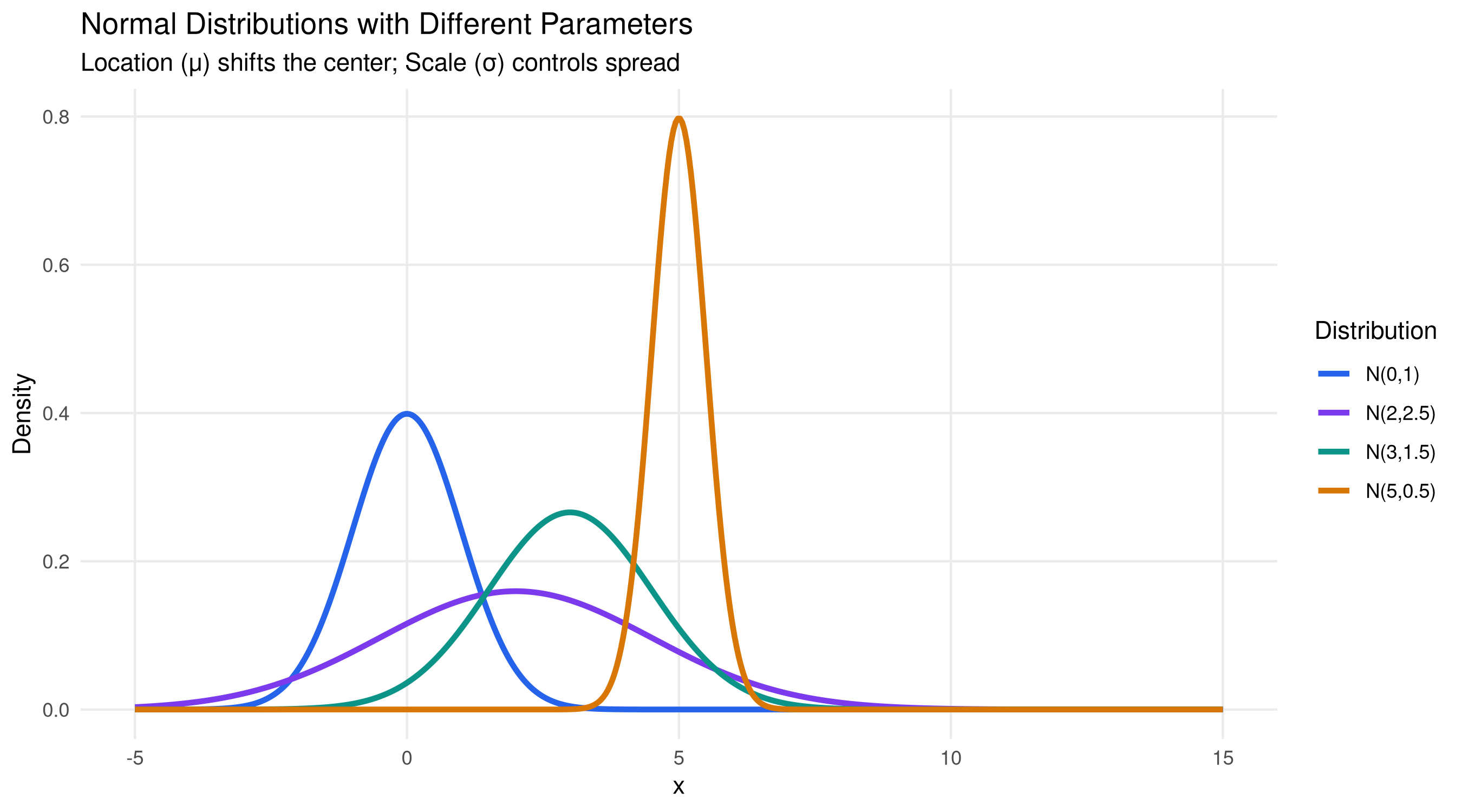
x <- seq(-4, 4, length.out=1000)
df_norm <- data.frame(x=x, y=dnorm(x))

ggplot(df_norm, aes(x,y)) +
  geom_area(data=filter(df_norm, x >= -3 & x <= 3), fill="#93c5fd", alpha=0.3) +
  geom_area(data=filter(df_norm, x >= -2 & x <= 2), fill="#60a5fa", alpha=0.4) +
  geom_area(data=filter(df_norm, x >= -1 & x <= 1), fill="#2563eb", alpha=0.5) +
  geom_line(linewidth=1.5, color="#1e3a8a") +
  geom_vline(xintercept=c(-3,-2,-1,0,1,2,3), linetype="dashed",
             alpha=0.4, color="#64748b") +
  annotate("text", x=0, y=0.2, label="68%\n(±1σ)", size=3.5, fontface="bold", color="white") +
  annotate("text", x=1.7, y=0.05, label="95%\n(±2σ)", size=3, color="#1e40af") +
  annotate("text", x=2.7, y=0.015, label="99.7%\n(±3σ)", size=2.5, color="#1e3a8a") +
  labs(title="Empirical Rule: 68-95-99.7",
       x="Standard Deviations from Mean", y="Density") +
  theme_minimal(base_size=11) +
  theme(panel.grid.minor=element_blank())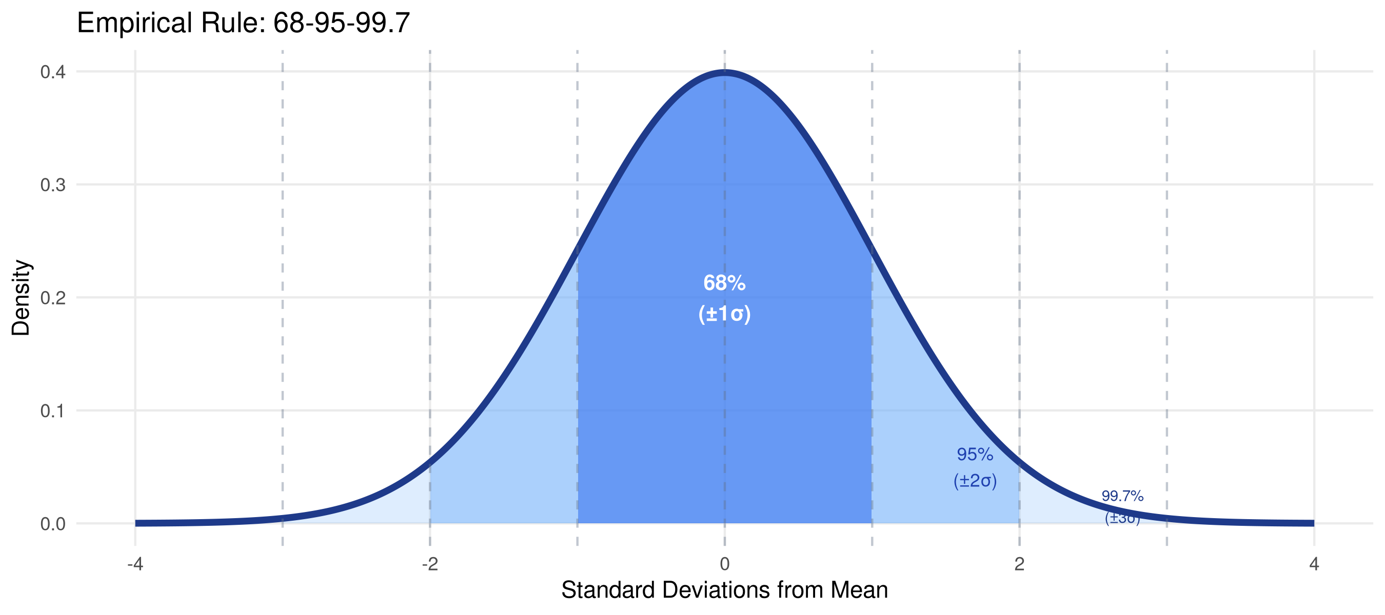
# Probability calculations
cat("P(Z ≤ 1.96)  =", round(pnorm(1.96), 4), "\n")
P(Z ≤ 1.96) = 0.975 cat("P(-1.96 ≤ Z ≤ 1.96) =", round(pnorm(1.96) - pnorm(-1.96), 4), "\n")P(-1.96 ≤ Z ≤ 1.96) = 0.95 cat("P(Z > 2.33) =", round(1 - pnorm(2.33), 4), "\n")P(Z > 2.33) = 0.0099 cat("95th percentile (z):", round(qnorm(0.95), 4), "\n")95th percentile (z): 1.6449 cat("99th percentile (z):", round(qnorm(0.99), 4), "\n")99th percentile (z): 2.3263 Used when we have n independent trials, each with probability p of success.
Application: In a survey of 100 households, if 35% own agricultural land, what’s the probability that exactly 40 own land?
n_trials <- 100
p_success <- 0.35

binom_df <- data.frame(
  k = 0:n_trials,
  prob = dbinom(0:n_trials, n_trials, p_success)
) |> filter(prob > 0.0001)

# Highlight specific outcomes
binom_df <- binom_df |>
  mutate(highlight = case_when(
    k == 40 ~ "k = 40",
    k >= 35 & k <= 40 ~ "35-40",
    TRUE ~ "Other"
  ))

ggplot(binom_df, aes(x=k, y=prob, fill=highlight)) +
  geom_col(width=0.7) +
  scale_fill_manual(values=c("k = 40"="#e11d48","35-40"="#7c3aed","Other"="#93c5fd"),
                    name="") +
  labs(title=paste0("Binomial(n=", n_trials, ", p=", p_success, ")"),
       x="Number of successes (k)", y="Probability P(X = k)") +
  theme_minimal(base_size=11) +
  theme(legend.position="top", panel.grid.minor=element_blank())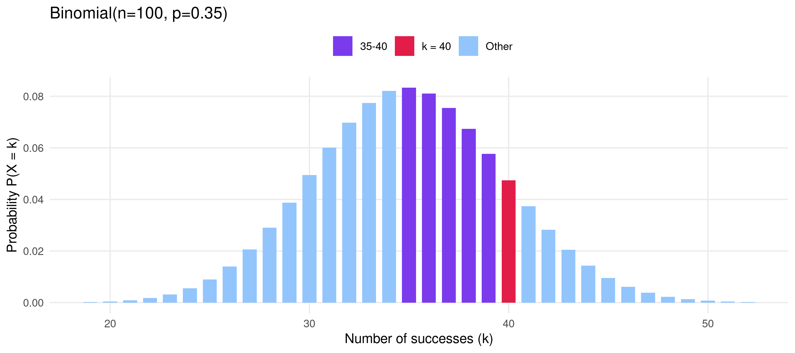
cat("P(X = 40) =", round(dbinom(40, 100, 0.35), 4))P(X = 40) = 0.0474cat("\nP(X ≥ 40) =", round(1 - pbinom(39, 100, 0.35), 4))
P(X ≥ 40) = 0.1724cat("\nExpected value E(X) = np =", 100*0.35)
Expected value E(X) = np = 35cat("\nSD(X) = √(np(1-p)) =", round(sqrt(100*0.35*0.65), 3))
SD(X) = √(np(1-p)) = 4.77Used for count data — events happening in a fixed interval.
Application: If a field surveyor visits an average of 8 households per hour, what’s the probability of visiting exactly 10 in an hour?
lambdas <- c(1, 3, 8, 15)
pois_df <- expand.grid(
  k = 0:30,
  lambda = lambdas
) |>
  mutate(
    prob  = dpois(k, lambda),
    label = paste0("λ = ", lambda)
  ) |> filter(prob > 0.001)

ggplot(pois_df, aes(x=k, y=prob, color=label)) +
  geom_line(linewidth=1.1) +
  geom_point(size=2) +
  scale_color_manual(values=c("#2563eb","#7c3aed","#0d9488","#d97706")) +
  labs(title="Poisson Distributions",
       x="k (count)", y="P(X = k)", color="Parameter") +
  theme_minimal(base_size=11) +
  theme(legend.position="right", panel.grid.minor=element_blank())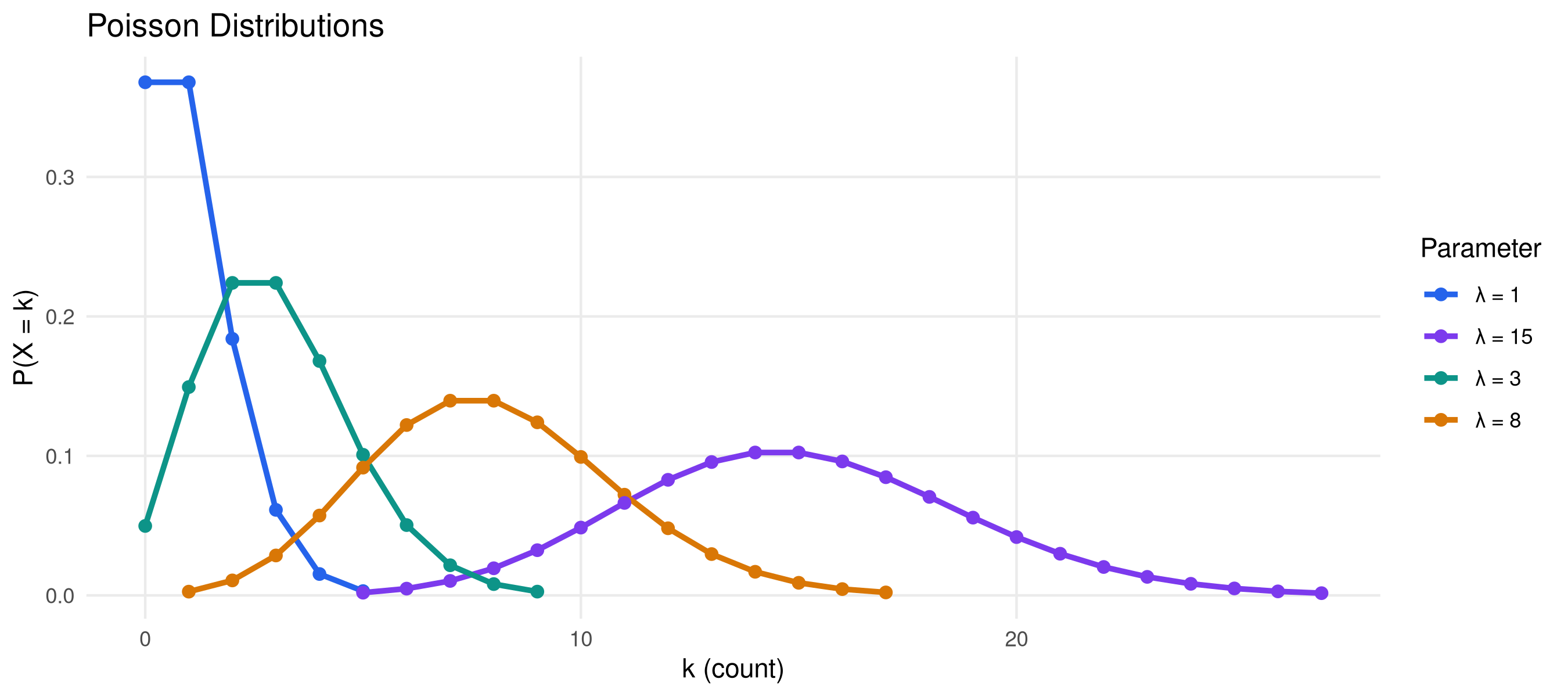
Used when the population standard deviation is unknown (which is almost always in practice).
x <- seq(-5, 5, length.out=500)
t_df <- bind_rows(
  data.frame(x=x, y=dnorm(x), dist="Normal (Z)"),
  data.frame(x=x, y=dt(x, df=3),  dist="t(df=3)"),
  data.frame(x=x, y=dt(x, df=10), dist="t(df=10)"),
  data.frame(x=x, y=dt(x, df=30), dist="t(df=30)")
)

ggplot(t_df, aes(x, y, color=dist, linetype=dist)) +
  geom_line(linewidth=1.1) +
  scale_color_manual(values=c("#0f172a","#e11d48","#7c3aed","#2563eb")) +
  scale_linetype_manual(values=c("dashed","solid","solid","solid")) +
  labs(title="t-Distribution vs Normal",
       subtitle="As df increases, t approaches the Standard Normal",
       x="x", y="Density", color="Distribution", linetype="Distribution") +
  theme_minimal(base_size=11) +
  theme(legend.position="right", panel.grid.minor=element_blank())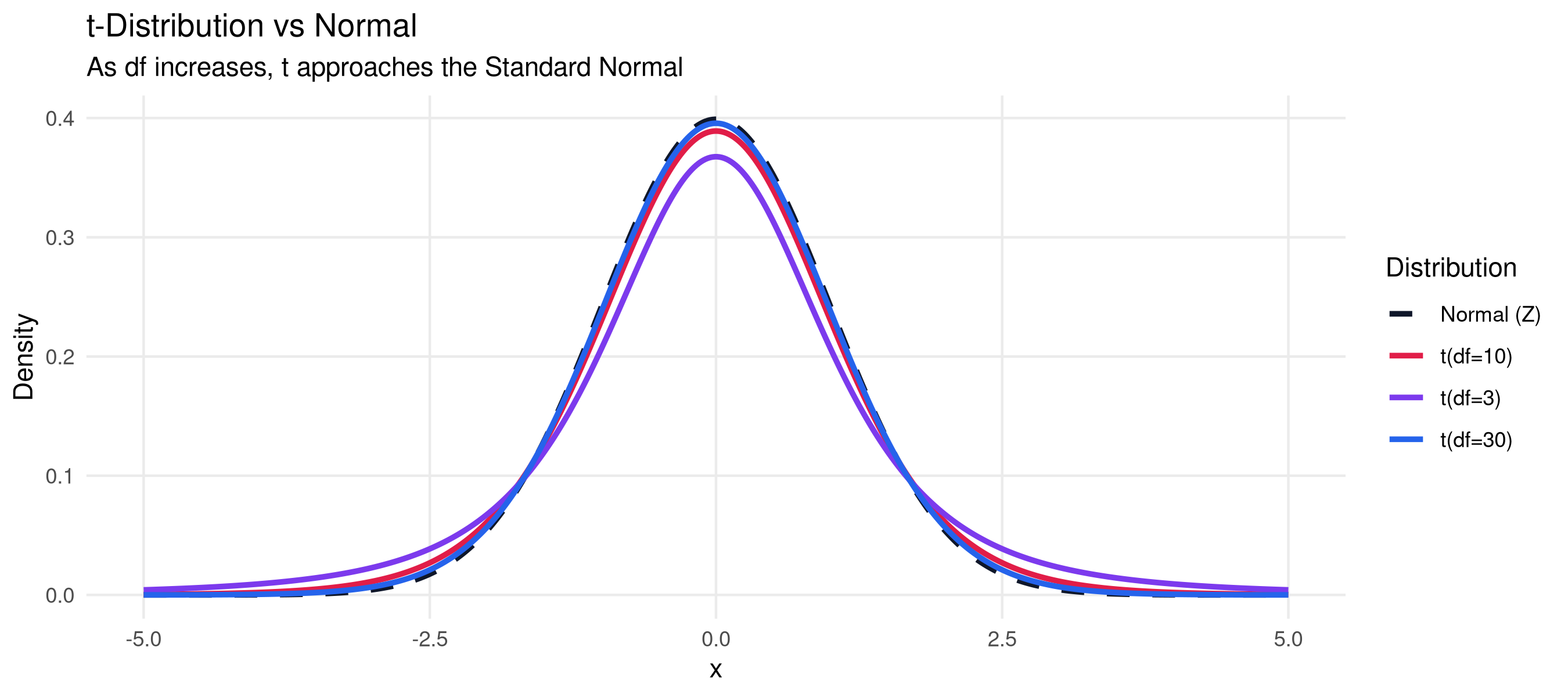
# Critical values
cat("t-critical values (two-tailed, α=0.05):\n")
t-critical values (two-tailed, α=0.05):for (df in c(5, 10, 20, 30, 60, 120)) {
cat(sprintf(" df=%3d: t = %.4f\n", df, qt(0.975, df)))
} df= 5: t = 2.5706
df= 10: t = 2.2281
df= 20: t = 2.0860
df= 30: t = 2.0423
df= 60: t = 2.0003
df=120: t = 1.9799cat(sprintf(" Normal: z = %.4f\n", qnorm(0.975))) Normal: z = 1.9600