---
title: "Beautiful Statistical Graphics with ggplot2"
description: "A step-by-step guide to creating publication-quality charts using ggplot2, including themes, annotations, and color scales."
author: "Pawan Jangra"
date: "2025-04-20"
categories: [R, ggplot2, Visualization]
image: "https://images.unsplash.com/photo-1460925895917-afdab827c52f?w=600&q=80"
toc: true
---
## Why ggplot2?
When I first switched from Excel to R for data visualization, ggplot2 felt confusing. "Why do I need `aes()`? What's a `geom`?" After years of use, I now think it's the most elegant visualization system ever designed.
The key insight is the **Grammar of Graphics**: every chart is built from composable layers.
## The Foundation: Data + Aesthetics + Geometry
```{r}
#| message: false
library(tidyverse)
library(scales)

# Create a realistic wage dataset
set.seed(2025)
wage_data <- data.frame(
  state     = rep(c("Haryana","Punjab","UP","Bihar","Maharashtra",
                    "Gujarat","Karnataka","Tamil Nadu"), each = 200),
  wage      = c(
    rnorm(200, 450, 80), rnorm(200, 480, 90), rnorm(200, 320, 70),
    rnorm(200, 280, 65), rnorm(200, 520, 110), rnorm(200, 490, 95),
    rnorm(200, 510, 100), rnorm(200, 535, 105)
  ),
  gender    = sample(c("Male","Female"), 1600, replace = TRUE, prob=c(.6,.4)),
  sector    = sample(c("Agriculture","Industry","Services"), 1600, replace=TRUE)
)
```
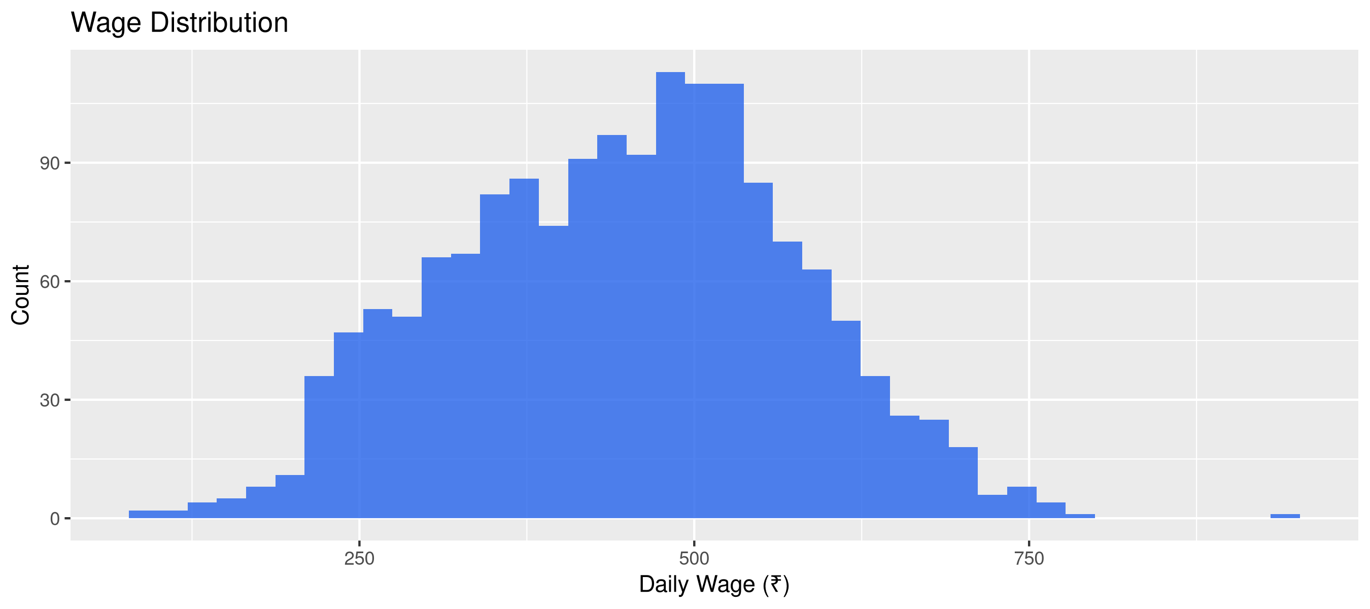
## Layer 1: The Basic Plot
```{r}
#| fig-height: 4
# Start simple
ggplot(wage_data, aes(x = wage)) +
  geom_histogram(bins = 40, fill = "#2563eb", alpha = 0.8) +
  labs(title = "Wage Distribution", x = "Daily Wage (₹)", y = "Count")
```
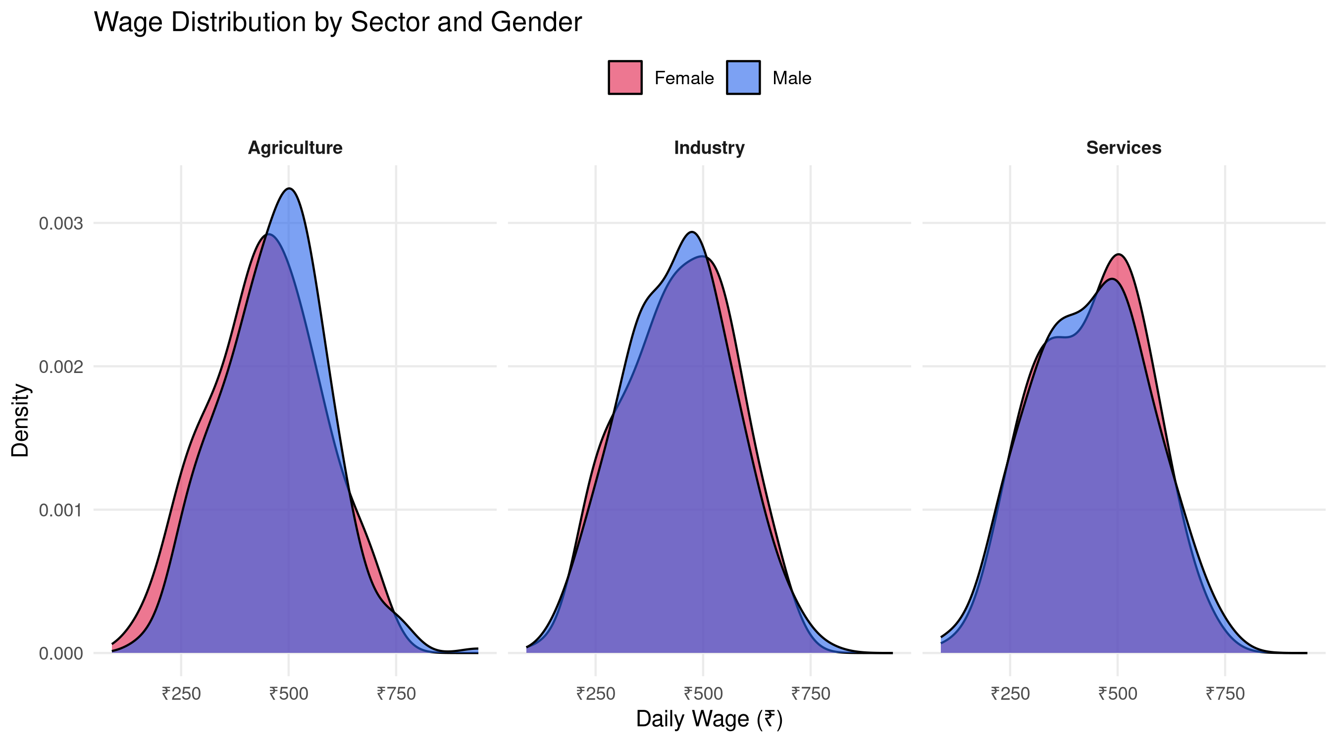
## Layer 2: Add Facets and Color
```{r}
#| fig-height: 5
ggplot(wage_data, aes(x = wage, fill = gender)) +
  geom_density(alpha = 0.6, adjust = 1.2) +
  facet_wrap(~sector, ncol = 3) +
  scale_fill_manual(values = c("Male"="#2563eb","Female"="#e11d48")) +
  scale_x_continuous(labels = label_number(prefix="₹")) +
  labs(title = "Wage Distribution by Sector and Gender",
       x = "Daily Wage (₹)", y = "Density", fill = NULL) +
  theme_minimal(base_size = 11) +
  theme(legend.position = "top",
        strip.text = element_text(face="bold"),
        panel.grid.minor = element_blank())
```
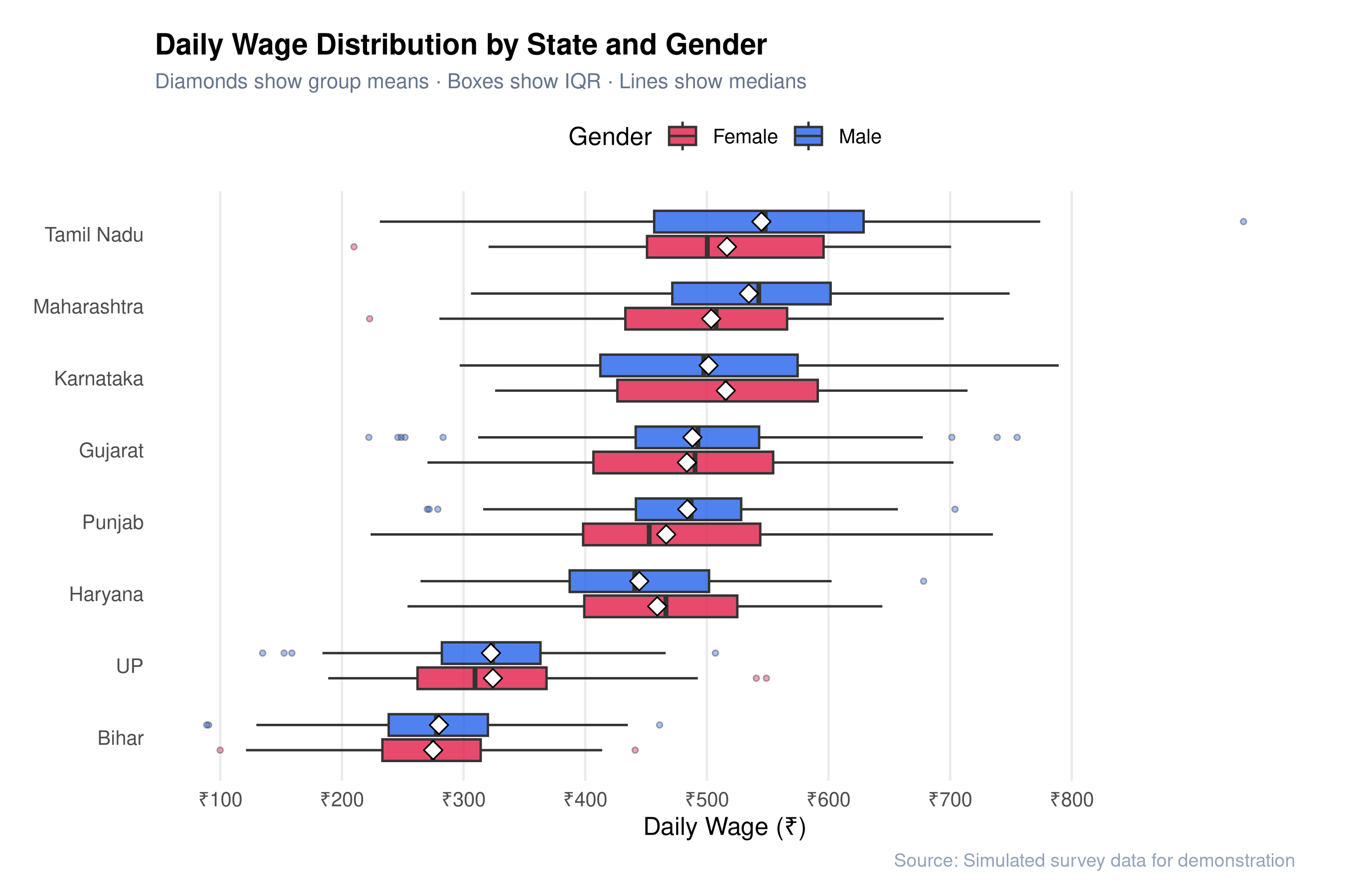
## Layer 3: Publication-Quality Box Plot
```{r}
#| fig-height: 6
#| fig-cap: "State-wise wage comparison — publication quality"
state_summary <- wage_data |>
  group_by(state) |>
  summarise(median_wage = median(wage), .groups = "drop") |>
  arrange(median_wage)

wage_data |>
  mutate(state = factor(state, levels = state_summary$state)) |>
  ggplot(aes(x = state, y = wage, fill = gender)) +
  geom_boxplot(
    outlier.shape = 21, outlier.size = 1, outlier.alpha = 0.4,
    width = 0.6, position = position_dodge(0.7), alpha = 0.8
  ) +
  stat_summary(
    aes(group = gender),
    fun = mean, geom = "point",
    shape = 23, size = 3, fill = "white",
    position = position_dodge(0.7)
  ) +
  scale_fill_manual(values = c("Male"="#2563eb","Female"="#e11d48"),
                    name = "Gender") +
  scale_y_continuous(
    labels = label_number(prefix = "₹"),
    breaks = seq(0, 800, 100)
  ) +
  coord_flip() +
  labs(
    title    = "Daily Wage Distribution by State and Gender",
    subtitle = "Diamonds show group means · Boxes show IQR · Lines show medians",
    x = NULL, y = "Daily Wage (₹)",
    caption  = "Source: Simulated survey data for demonstration"
  ) +
  theme_minimal(base_size = 12) +
  theme(
    plot.title       = element_text(face = "bold", size = 14),
    plot.subtitle    = element_text(color = "#64748b", size = 10),
    plot.caption     = element_text(color = "#94a3b8", size = 9),
    panel.grid.major.y = element_blank(),
    panel.grid.minor   = element_blank(),
    legend.position    = "top",
    plot.background    = element_rect(fill = "white", color = NA),
    plot.margin        = margin(16, 24, 12, 16)
  )
```
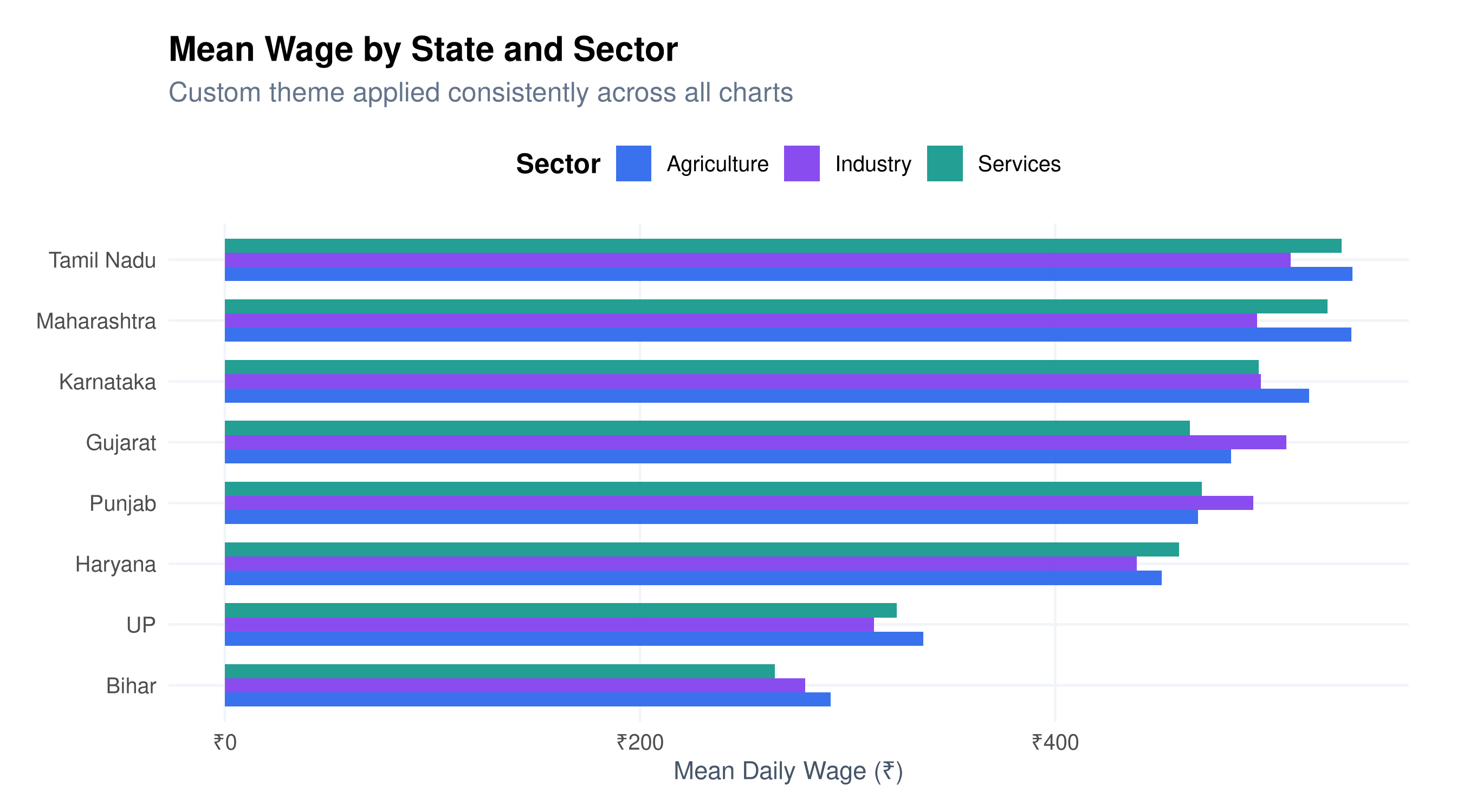
## Layer 4: Custom Theme Function
The real power comes from creating your own reusable theme:
```{r}
#| fig-height: 5
theme_pawan <- function(base_size = 12) {
  theme_minimal(base_size = base_size) +
    theme(
      text              = element_text(family = "sans"),
      plot.title        = element_text(face = "bold", size = base_size + 3, hjust = 0),
      plot.subtitle     = element_text(color = "#64748b", hjust = 0, margin = margin(b = 10)),
      plot.caption      = element_text(color = "#94a3b8", size = base_size - 3, hjust = 1),
      panel.grid.minor  = element_blank(),
      panel.grid.major  = element_line(color = "#f1f5f9"),
      axis.title        = element_text(color = "#475569", size = base_size - 1),
      legend.position   = "top",
      legend.title      = element_text(face = "bold"),
      plot.background   = element_rect(fill = "white", color = NA),
      plot.margin       = margin(16, 24, 12, 16)
    )
}

# Use it
wage_data |>
  group_by(state, sector) |>
  summarise(mean_wage = mean(wage), .groups = "drop") |>
  ggplot(aes(x = reorder(state, mean_wage), y = mean_wage, fill = sector)) +
  geom_col(position = "dodge", width = 0.7, alpha = 0.9) +
  scale_fill_manual(values = c("#2563eb","#7c3aed","#0d9488")) +
  scale_y_continuous(labels = label_number(prefix = "₹")) +
  coord_flip() +
  labs(title = "Mean Wage by State and Sector",
       subtitle = "Custom theme applied consistently across all charts",
       x = NULL, y = "Mean Daily Wage (₹)", fill = "Sector") +
  theme_pawan()
```
The `theme_pawan()` function means every chart in a report looks consistent — a crucial detail for professional work.