---
title: "Sampling Methods in Field Research: What I Learned"
description: "From stratified to cluster sampling — practical insights from 7 years of field survey work across India."
author: "Pawan Jangra"
date: "2025-05-10"
categories: [Survey, Statistics, Field Research]
image: "https://images.unsplash.com/photo-1454165804606-c3d57bc86b40?w=600&q=80"
toc: true
---
## The Reality of Field Sampling
Textbooks make sampling sound clean. Reality is messier. In my years of field survey work — from rural Haryana to urban Maharashtra — I've encountered almost every challenge sampling theory describes, plus a few it doesn't.
This post is my attempt to bridge the theory-practice gap.
## Simple Random Sampling: Rarely Simple in Practice
```{r}
#| message: false
library(tidyverse)

# Simulate a village population
set.seed(42)
village_pop <- data.frame(
  household_id = 1:500,
  income = exp(rnorm(500, log(8000), 0.8)),
  num_members = rpois(500, 4.5) + 1,
  landholding = rexp(500, 1/2.5)  # acres
)

# SRS: draw 50 households
srs_sample <- village_pop |>
  slice_sample(n = 50)

# Compare estimates to true values
comparison <- bind_rows(
  village_pop |> summarise(group = "Population",
                           mean_income = mean(income),
                           mean_size = mean(num_members)),
  srs_sample |> summarise(group = "SRS Sample (n=50)",
                           mean_income = mean(income),
                           mean_size = mean(num_members))
)

knitr::kable(comparison, digits = 1,
             caption = "SRS vs Population parameters")
```
The estimates are close — but in field reality, SRS requires a complete sampling frame (list of all households), which rarely exists in rural areas.
## Stratified Sampling: My Preferred Approach
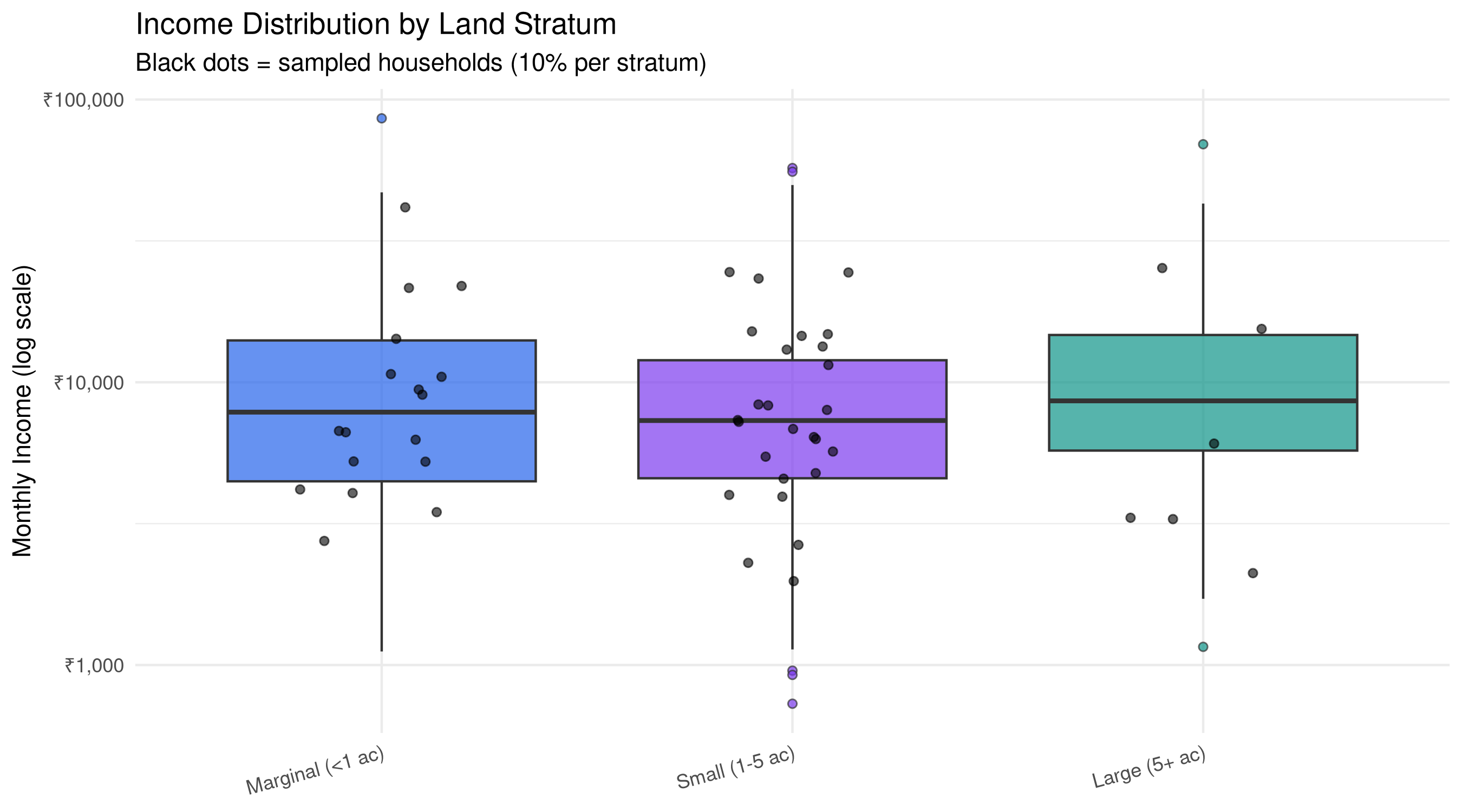
When I joined SSER, we almost always used stratified sampling for district-level surveys. Here's why it works:
```{r}
#| fig-height: 5
# Add strata based on landholding
village_pop <- village_pop |>
  mutate(
    stratum = case_when(
      landholding == 0         ~ "Landless",
      landholding < 1          ~ "Marginal (<1 ac)",
      landholding < 5          ~ "Small (1-5 ac)",
      TRUE                     ~ "Large (5+ ac)"
    ) |> factor(levels = c("Landless","Marginal (<1 ac)","Small (1-5 ac)","Large (5+ ac)"))
  )

# Proportional stratified sample
strat_sample <- village_pop |>
  group_by(stratum) |>
  slice_sample(prop = 0.1) |>  # 10% from each stratum
  ungroup()

# Visualise income by stratum
ggplot(village_pop, aes(x = stratum, y = income, fill = stratum)) +
  geom_boxplot(alpha = 0.7, outlier.shape = 21) +
  geom_jitter(data = strat_sample, aes(x = stratum, y = income),
              width = 0.2, alpha = 0.6, color = "black", size = 1.5) +
  scale_y_log10(labels = scales::label_number(prefix = "₹", big.mark = ",")) +
  scale_fill_manual(values = c("#2563eb","#7c3aed","#0d9488","#d97706")) +
  labs(title = "Income Distribution by Land Stratum",
       subtitle = "Black dots = sampled households (10% per stratum)",
       x = NULL, y = "Monthly Income (log scale)") +
  theme_minimal(base_size = 11) +
  theme(legend.position = "none",
        axis.text.x = element_text(angle = 15, hjust = 1))
```
## Cluster Sampling: Practical but Tricky
Cluster sampling is often the only feasible approach for large geographic surveys. We used it extensively when surveying across multiple districts.
```{r}
# Simulate 20 clusters (villages), sample 5 clusters
set.seed(99)
n_clusters <- 20
clusters <- data.frame(
  cluster_id = 1:n_clusters,
  district = sample(c("Rohtak","Hisar","Karnal","Panipat"),
                    n_clusters, replace = TRUE),
  pop_size = sample(200:800, n_clusters)
)

# Within-cluster correlation (ICC) effect
icc <- 0.15  # typical for income surveys
design_effect <- 1 + (mean(clusters$pop_size) - 1) * icc

cat("Design Effect (DEFF):", round(design_effect, 2))
cat("\nEffective sample size reduction:", round((1 - 1/design_effect)*100, 1), "%")
```
**The key lesson:** Always account for the design effect when reporting standard errors from cluster samples. Ignoring it gives you artificially small standard errors and overconfident conclusions.
## Practical Tips from the Field
1. **Listing comes first** — Before sampling, build your sampling frame carefully. In rural areas, this often means a fresh household listing exercise.
2. **Replacement rules matter** — Define substitution procedures before going to field. What happens when a sampled household is locked or refuses?
3. **Random starts in systematic sampling** — Always use a random start for systematic samples, not just household #1.
4. **Weight your data** — After collecting, compute and apply sampling weights before any analysis. The `survey` package in R handles this beautifully.
Field sampling is as much art as science. The best designs balance statistical efficiency with logistical feasibility.