---
title: "Data Wrangling with tidyverse: A Practical Guide"
description: "Learn how to efficiently wrangle messy datasets using dplyr, tidyr, and readr with real-world survey data examples."
author: "Pawan Jangra"
date: "2025-06-15"
categories: [R, Tidyverse, Data Cleaning]
image: "https://images.unsplash.com/photo-1551288049-bebda4e38f71?w=600&q=80"
toc: true
---
## Introduction
After years of working with messy survey data — from PLFS datasets to field-collected ODK forms — I've come to appreciate how the `tidyverse` ecosystem makes data wrangling not just efficient, but almost enjoyable. This post shares the patterns I use most often.
## Setting Up
```{r}
#| message: false
library(tidyverse)
library(knitr)

# Simulate a messy survey dataset
set.seed(2025)
n <- 200

raw_survey <- data.frame(
  id         = 1:n,
  age        = sample(c(18:80, NA), n, replace = TRUE,
                      prob = c(rep(1, 63), rep(5, 1))),
  income     = paste0("₹", round(runif(n, 5000, 150000), -2)),
  gender     = sample(c("M", "F", "male", "female", "MALE", "1", "2", NA),
                      n, replace = TRUE),
  state      = sample(c("HR", "PB", "UP", "BR", "MH", NA), n, replace = TRUE),
  employment = sample(c("Employed", "Unemployed", "Self-Employed",
                         "employed", "NA", NA), n, replace = TRUE)
)

glimpse(raw_survey)
```
## Step 1: Standardise Text Variables
One of the most common issues in field surveys is inconsistent coding. Here's how to fix it cleanly:
```{r}
clean_survey <- raw_survey |>
  # Standardise gender
  mutate(
    gender_clean = case_when(
      str_to_lower(gender) %in% c("m", "male", "1") ~ "Male",
      str_to_lower(gender) %in% c("f", "female", "2") ~ "Female",
      .default = NA_character_
    ),
    # Clean income: remove ₹ symbol and convert to numeric
    income_num = as.numeric(str_remove(income, "₹")),
    # Standardise employment
    employment_clean = case_when(
      str_to_lower(employment) == "employed"      ~ "Employed",
      str_to_lower(employment) == "unemployed"    ~ "Unemployed",
      str_to_lower(employment) == "self-employed" ~ "Self-Employed",
      .default = NA_character_
    )
  )

# Check results
clean_survey |>
  count(gender_clean) |>
  kable(caption = "Gender distribution after cleaning")
```
## Step 2: Handle Missing Values
```{r}
# Check missingness
miss_summary <- clean_survey |>
  summarise(across(everything(), ~sum(is.na(.)))) |>
  pivot_longer(everything(), names_to = "variable", values_to = "missing") |>
  mutate(pct_missing = round(missing / n * 100, 1)) |>
  arrange(desc(missing))

kable(miss_summary, caption = "Missing value summary")
```
## Step 3: Create Summary Tables
```{r}
# Age-Income analysis by gender
summary_table <- clean_survey |>
  filter(!is.na(gender_clean), !is.na(income_num)) |>
  group_by(gender_clean, state) |>
  summarise(
    n          = n(),
    mean_age   = round(mean(age, na.rm = TRUE), 1),
    mean_income = round(mean(income_num, na.rm = TRUE)),
    median_income = median(income_num, na.rm = TRUE),
    .groups = "drop"
  ) |>
  arrange(state, gender_clean)

kable(summary_table,
      caption = "Summary statistics by gender and state",
      format.args = list(big.mark = ","))
```
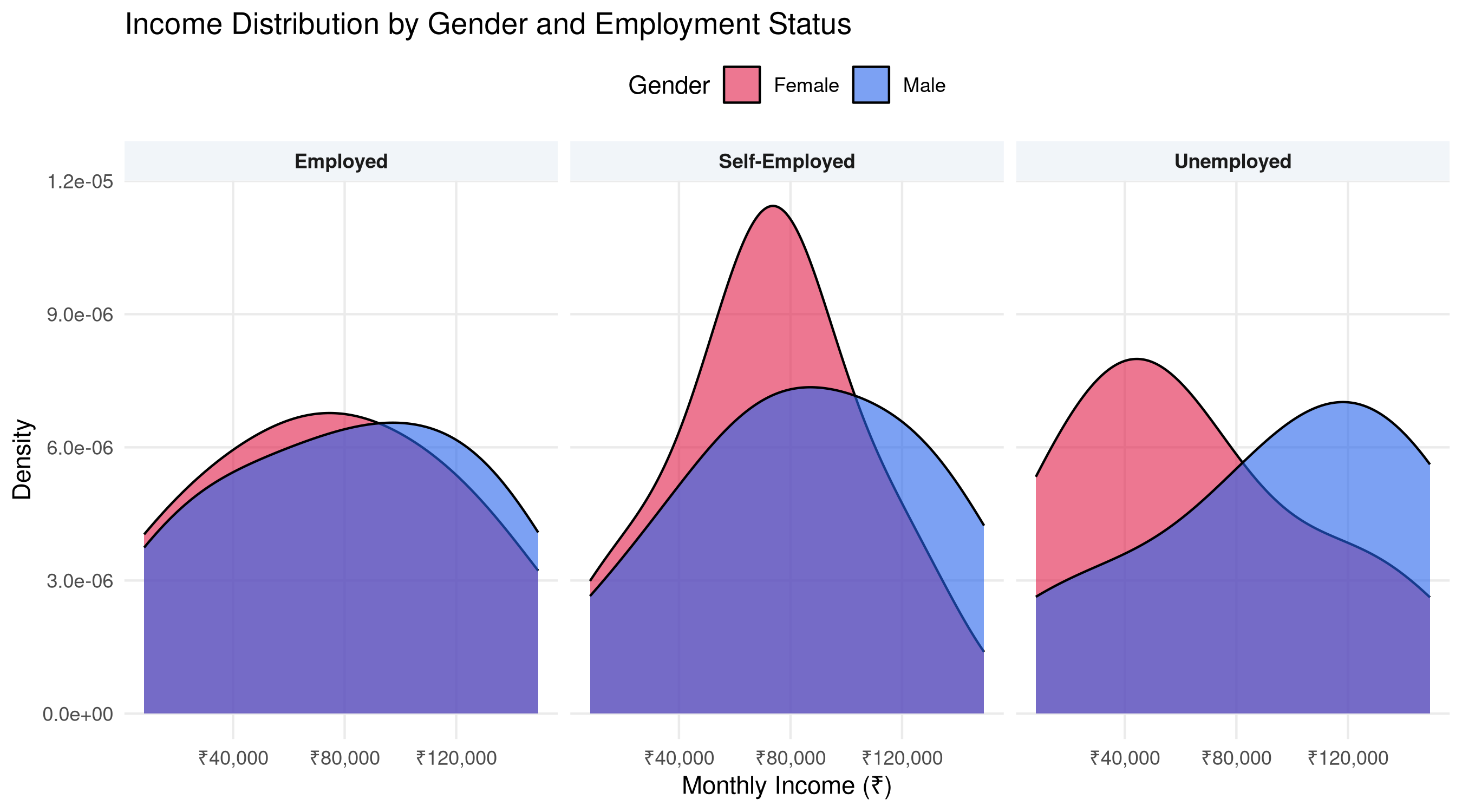
## Step 4: Visualise the Clean Data
```{r}
#| fig-height: 5
#| fig-cap: "Income distribution by gender and employment status"
clean_survey |>
  filter(!is.na(gender_clean), !is.na(employment_clean), !is.na(income_num)) |>
  ggplot(aes(x = income_num, fill = gender_clean)) +
  geom_density(alpha = 0.6, adjust = 1.5) +
  facet_wrap(~employment_clean) +
  scale_x_continuous(labels = scales::label_number(prefix = "₹", big.mark = ",")) +
  scale_fill_manual(values = c("Male" = "#2563eb", "Female" = "#e11d48")) +
  labs(
    title = "Income Distribution by Gender and Employment Status",
    x = "Monthly Income (₹)", y = "Density", fill = "Gender"
  ) +
  theme_minimal(base_size = 11) +
  theme(
    strip.background = element_rect(fill = "#f1f5f9", color = NA),
    strip.text = element_text(face = "bold"),
    panel.grid.minor = element_blank(),
    legend.position = "top"
  )
```
## Key Takeaways
The `tidyverse` pipeline (`|>`) allows you to chain data transformations in a readable, logical sequence. The key principles I follow:
1. **Never modify raw data** — always create a new `clean_` object
2. **Standardise early** — fix encoding, case, and symbols before any analysis
3. **Document decisions** — use `# comments` to explain why you made choices
4. **Check your work** — use `count()` and `glimpse()` frequently
In my next post, I'll cover how to handle survey weights using the `survey` package in R.