Statistical Graphics

Visualising Data Effectively in R

Author

Pawan

Published

May 11, 2026

Introduction

Statistical graphics are visual representations of data that help us explore distributions, relationships, patterns, and anomalies that are impossible to see in tables of numbers.

“A picture is worth a thousand words — in statistics, a good chart is worth a thousand rows of data.”

Good graphics are the first and last step in data analysis: used in exploratory data analysis (EDA) to understand data, and in reporting to communicate findings.

Principles of Good Statistical Graphics

Show the data: Do not hide information with over-aggregation.
Maximise data-ink ratio: Remove non-essential decorations (chart junk).
Label clearly: Every axis, title, and legend must be informative.
Choose the right chart: The chart type must match the data type and the question.
Avoid misleading scales: Always start y-axis at 0 for bar charts.

Choosing the Right Chart

Data Type	Comparison Goal	Best Chart
One continuous variable	Distribution	Histogram, Density, Boxplot
One categorical variable	Frequency	Bar chart, Pie chart
Two continuous variables	Relationship	Scatter plot
Continuous over time	Trend	Line chart
Continuous by category	Comparison	Side-by-side boxplot
Multivariate	Overview	Pairs plot, Heatmap
Part-to-whole	Proportion	Stacked bar, Pie

Base R Graphics

Setup

data(mtcars)
data(iris)

# Convert cyl to factor for grouped plots
mtcars$cyl <- as.factor(mtcars$cyl)

Histogram — Distribution of One Variable

hist(mtcars$mpg,
     breaks = 12,
     col    = "steelblue",
     border = "white",
     main   = "Distribution of Fuel Efficiency",
     xlab   = "Miles Per Gallon (MPG)",
     ylab   = "Frequency")

# Add density curve
lines(density(mtcars$mpg) |> (\(d) list(x = d$x, y = d$y * length(mtcars$mpg) * diff(range(mtcars$mpg)) / 12))(),
      col = "red", lwd = 2)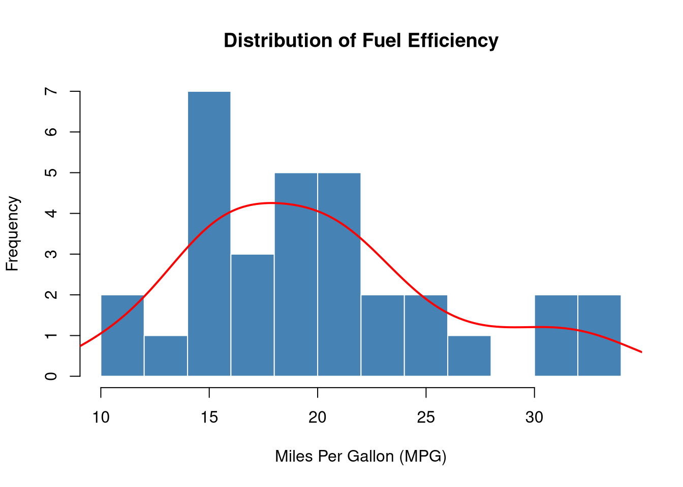

When to use: To see the shape, spread, and central tendency of a single continuous variable.

Boxplot — Comparing Distributions

boxplot(mpg ~ cyl,
        data   = mtcars,
        col    = c("lightblue", "lightgreen", "salmon"),
        border = "navy",
        main   = "MPG by Number of Cylinders",
        xlab   = "Cylinders",
        ylab   = "Miles Per Gallon")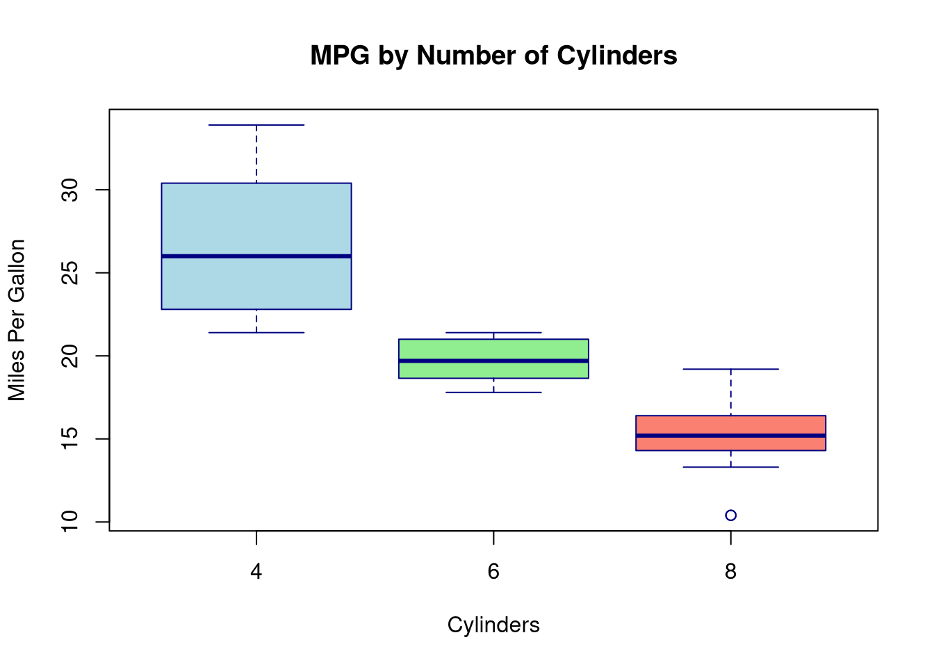

Reading a boxplot:

Box: Q1 to Q3 (middle 50% of data)
Line inside box: Median (Q2)
Whiskers: Extend to 1.5 × IQR from the box edges
Points beyond whiskers: Outliers

When to use: Compare distributions across groups; excellent for detecting outliers.

Scatter Plot — Relationship Between Two Variables

plot(mtcars$wt, mtcars$mpg,
     pch  = 16,
     col  = as.numeric(mtcars$cyl) + 1,
     cex  = 1.3,
     xlab = "Weight (1000 lbs)",
     ylab = "Miles Per Gallon",
     main = "Weight vs MPG by Cylinders")

legend("topright",
       legend = c("4 cyl", "6 cyl", "8 cyl"),
       col    = c(2, 3, 4),
       pch    = 16,
       title  = "Cylinders")

# Add overall trend line
abline(lm(mpg ~ wt, data = mtcars), col = "darkgrey", lwd = 2, lty = 2)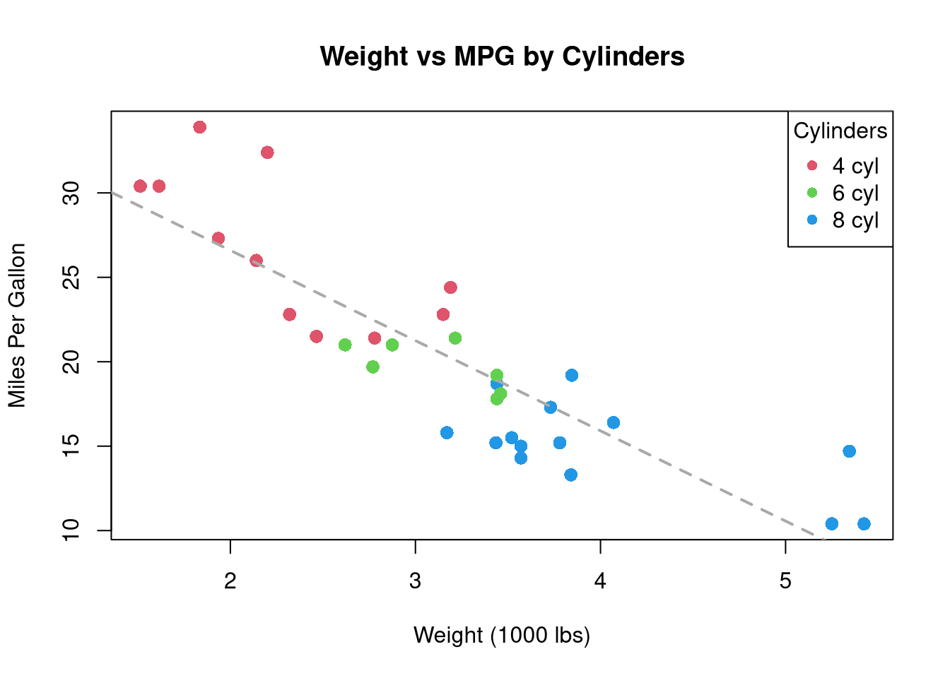

When to use: Examine the relationship (direction, strength, linearity) between two continuous variables.

Bar Chart — Frequency of Categories

cyl_counts <- table(mtcars$cyl)

barplot(cyl_counts,
        col    = c("lightblue", "steelblue", "navy"),
        border = "white",
        main   = "Number of Cars by Cylinder Count",
        xlab   = "Cylinders",
        ylab   = "Count",
        ylim   = c(0, 16))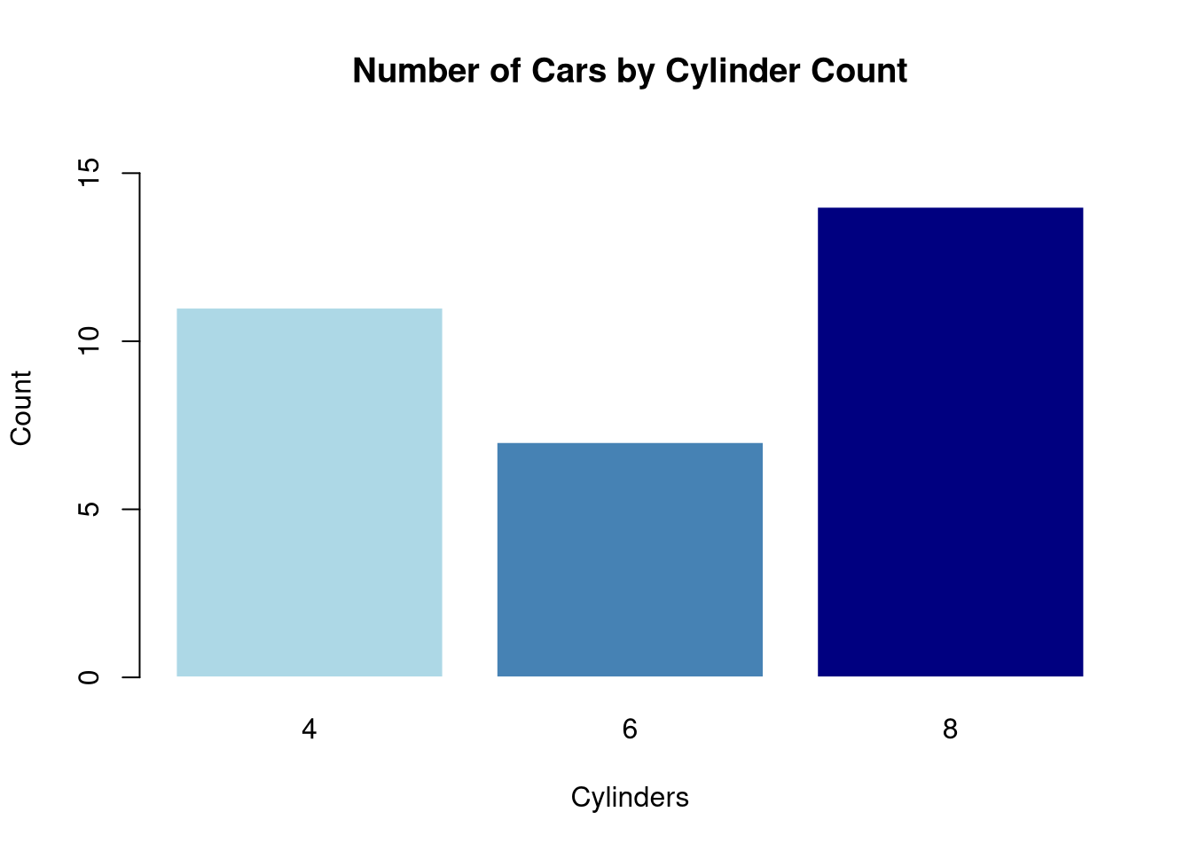

When to use: Show counts or frequencies for categorical data.

Line Chart — Trends Over Time

plot(AirPassengers,
     col  = "steelblue",
     lwd  = 2,
     main = "Monthly Airline Passengers (1949–1960)",
     xlab = "Year",
     ylab = "Passengers (thousands)")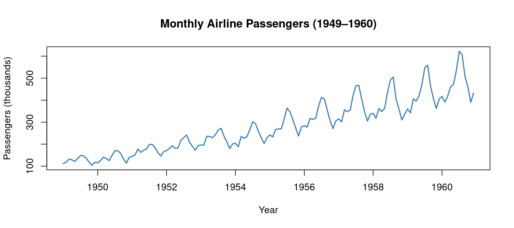

When to use: Display how a quantity changes over time.

Pairs Plot — Multivariate Overview

pairs(iris[, 1:4],
      col  = as.numeric(iris$Species) + 1,
      pch  = 16,
      main = "Pairs Plot — Iris Dataset",
      labels = c("Sepal\nLength", "Sepal\nWidth", "Petal\nLength", "Petal\nWidth"))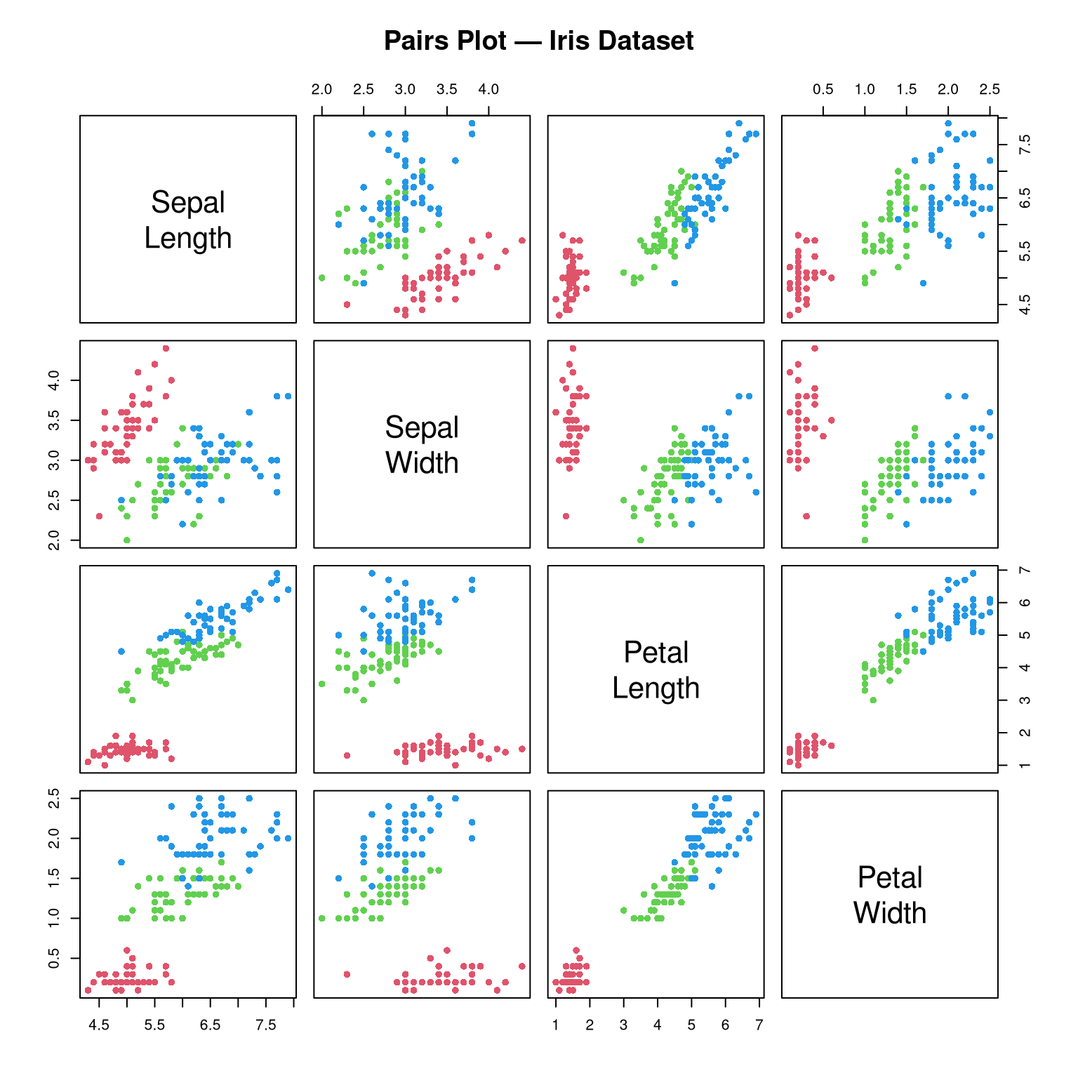

When to use: Explore all pairwise relationships in a dataset simultaneously. Excellent for EDA.

ggplot2 — Grammar of Graphics

ggplot2 is based on the Grammar of Graphics: every plot is built from:

Data: the dataset
Aesthetics (aes): what variables map to x, y, colour, size, shape
Geometries (geom_*): the visual elements (points, lines, bars, boxes)
Scales: control axes and legends
Facets: split into subplots
Theme: control the non-data appearance

ggplot(data, aes(x = ..., y = ..., colour = ...)) +
  geom_*() +
  labs(...) +
  theme_*()

Setup

# install.packages("ggplot2")
library(ggplot2)

# Convert for ggplot
mtcars2 <- mtcars
mtcars2$cyl <- as.factor(mtcars2$cyl)

ggplot2 Histogram

ggplot(mtcars2, aes(x = mpg)) +
  geom_histogram(bins = 12, fill = "steelblue", colour = "white") +
  geom_density(aes(y = after_stat(count) * 2.5),
               colour = "red", linewidth = 1) +
  labs(title = "Distribution of MPG",
       x = "Miles Per Gallon",
       y = "Count") +
  theme_minimal()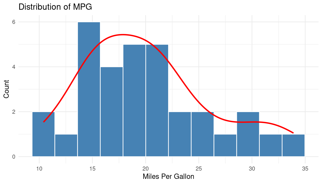

ggplot2 Boxplot

ggplot(mtcars2, aes(x = cyl, y = mpg, fill = cyl)) +
  geom_boxplot(outlier.colour = "red", outlier.shape = 16) +
  scale_fill_manual(values = c("lightblue", "lightgreen", "salmon")) +
  labs(title = "MPG Distribution by Cylinders",
       x = "Number of Cylinders",
       y = "Miles Per Gallon",
       fill = "Cylinders") +
  theme_minimal() +
  theme(legend.position = "none")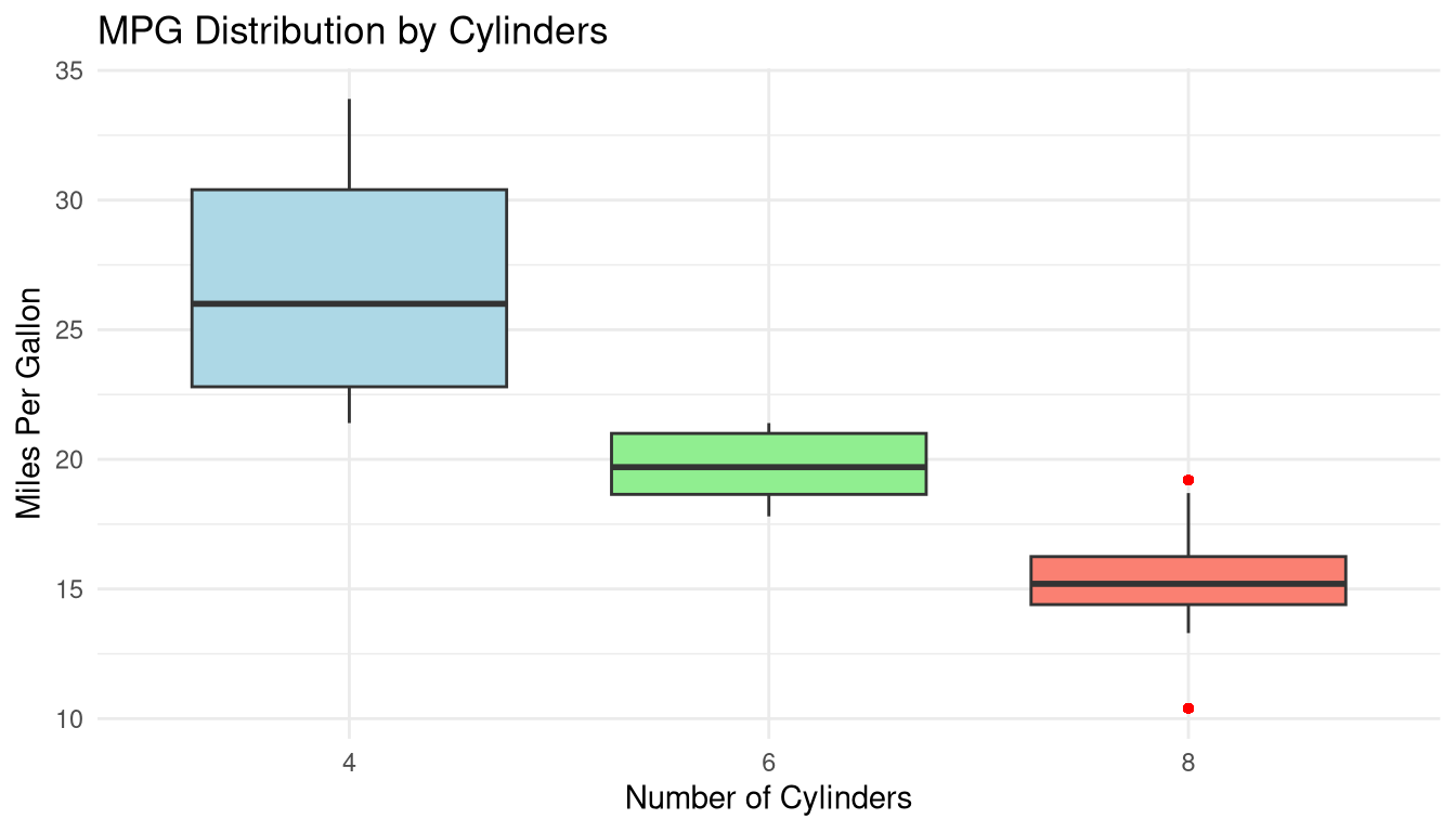

ggplot2 Scatter Plot with Smooth Trend

ggplot(mtcars2, aes(x = wt, y = mpg, colour = cyl)) +
  geom_point(size = 3, alpha = 0.8) +
  geom_smooth(method = "lm", se = TRUE, colour = "black",
              linetype = "dashed", linewidth = 0.8) +
  scale_colour_manual(values = c("4" = "#2196F3",
                                  "6" = "#4CAF50",
                                  "8" = "#F44336")) +
  labs(title    = "Weight vs MPG",
       subtitle = "Linear trend with 95% confidence band",
       x        = "Weight (1000 lbs)",
       y        = "Miles Per Gallon",
       colour   = "Cylinders") +
  theme_minimal()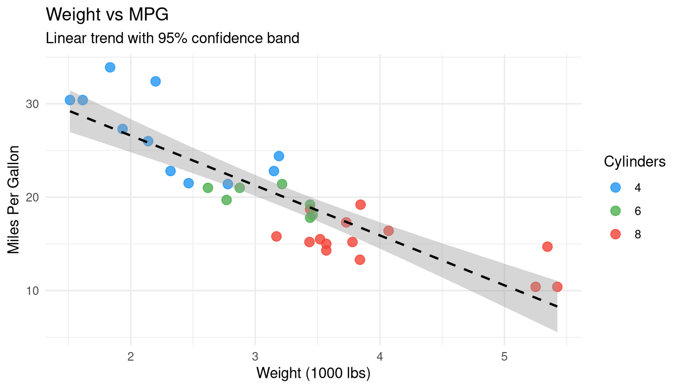

ggplot2 Faceted Plot

ggplot(mtcars2, aes(x = wt, y = mpg)) +
  geom_point(colour = "steelblue", size = 2.5, alpha = 0.8) +
  geom_smooth(method = "lm", se = FALSE, colour = "red") +
  facet_wrap(~ cyl, labeller = label_both) +
  labs(title = "MPG vs Weight — Faceted by Cylinders",
       x = "Weight (1000 lbs)",
       y = "Miles Per Gallon") +
  theme_bw()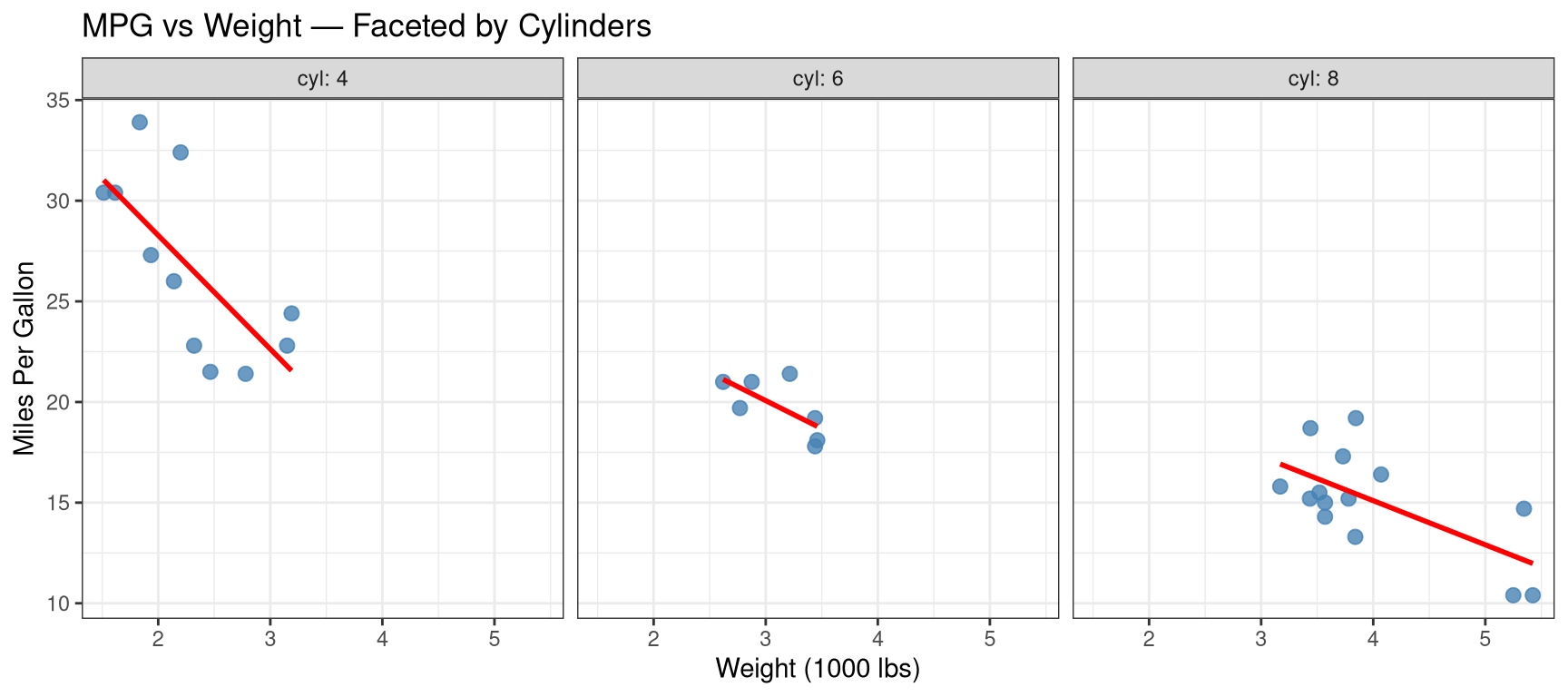

When to use facets: Compare the same relationship across subgroups without overlapping data.

ggplot2 Bar Chart

ggplot(mtcars2, aes(x = cyl, fill = cyl)) +
  geom_bar() +
  scale_fill_manual(values = c("lightblue", "steelblue", "navy")) +
  labs(title = "Car Count by Cylinders",
       x = "Cylinders", y = "Count") +
  theme_minimal() +
  theme(legend.position = "none")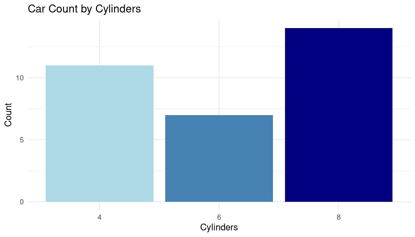

Heatmap — Correlation Matrix

# Compute correlation matrix
mtcars_num <- mtcars[, sapply(mtcars, is.numeric)]
cor_mat <- cor(mtcars_num)

# Reshape for ggplot
cor_df <- as.data.frame(as.table(cor_mat))
names(cor_df) <- c("Var1", "Var2", "Correlation")

ggplot(cor_df, aes(x = Var1, y = Var2, fill = Correlation)) +
  geom_tile(colour = "white", linewidth = 0.5) +
  geom_text(aes(label = round(Correlation, 2)),
            size = 3, colour = "black") +
  scale_fill_gradient2(low = "#D73027", mid = "white", high = "#1A9850",
                       midpoint = 0, limits = c(-1, 1)) +
  labs(title = "Correlation Heatmap — mtcars",
       x = "", y = "") +
  theme_minimal() +
  theme(axis.text.x = element_text(angle = 45, hjust = 1))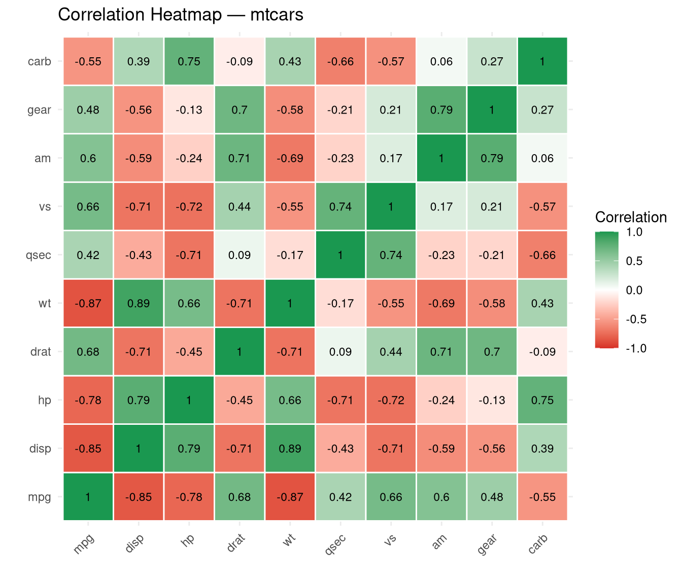

When to use: Quickly identify strongly correlated variable pairs before regression modelling.

Saving Plots

# Base R
png("my_plot.png", width = 800, height = 600)
hist(mtcars$mpg)
dev.off()

# ggplot2
p <- ggplot(mtcars2, aes(x = mpg)) + geom_histogram(fill = "steelblue")
ggsave("my_ggplot.png", plot = p, width = 8, height = 5, dpi = 300)

Summary

Chart Type	Best For	Base R	ggplot2
Histogram	Distribution	`hist()`	`geom_histogram()`
Boxplot	Comparing groups	`boxplot()`	`geom_boxplot()`
Scatter	Relationships	`plot()`	`geom_point()`
Bar chart	Frequencies	`barplot()`	`geom_bar()`
Line chart	Time trends	`plot()` with `type="l"`	`geom_line()`
Pairs plot	Multivariate EDA	`pairs()`	`GGally::ggpairs()`
Heatmap	Correlations	`heatmap()`	`geom_tile()`
Density	Smooth distribution	`density()` + `plot()`	`geom_density()`

Statistical graphics are not decoration — they are the primary tool for discovering structure in data. Always plot before modelling, and always plot your results.