Pawan.
  • About
  • Experience
  • Content Hub
  • Skills
  • Editor
  • R Code
  • Contact

On this page

  • Introduction
  • Components of a Time Series
    • Decomposition Models
  • Key Concepts and Definitions
    • Stationarity
    • Autocorrelation Function (ACF)
    • Partial Autocorrelation Function (PACF)
  • The ARIMA Family of Models
    • AR(p) — Autoregressive Model
    • MA(q) — Moving Average Model
    • ARMA(p, q)
    • ARIMA(p, d, q)
      • Model Selection Guide
  • When and Where to Use Time Series Models
  • Implementation in R
    • Loading a Time Series
    • Plotting the Series
    • Decomposition
    • Stationarity Testing — Augmented Dickey-Fuller Test
    • ACF and PACF Plots
    • Fitting ARIMA Model
    • Auto-ARIMA (automatic order selection)
    • Forecasting
    • Checking Residuals
    • Accuracy Metrics
    • Exponential Smoothing (ETS) — Alternative Approach
  • Summary
  • Report an issue

Other Formats

  • PDF

Time Series Models

Analysis, Decomposition, and Forecasting in R

Author

Pawan

Published

May 11, 2026

Introduction

A time series is a sequence of data points collected at successive points in time, typically at equally spaced intervals. Time series analysis is used to understand past behaviour and forecast future values.

Examples: monthly rainfall, daily stock prices, quarterly GDP, weekly sales figures, annual temperature records.


Components of a Time Series

Every time series can be decomposed into four components:

Component Symbol Description
Trend (\(T_t\)) Long-run direction Rising, falling, or flat over time
Seasonality (\(S_t\)) Regular periodic pattern Repeats within a known period (month, quarter, year)
Cyclical (\(C_t\)) Long-term wave Multi-year business/economic cycles
Irregular/Noise (\(I_t\)) Random fluctuation Unexplained random variation

Decomposition Models

Additive model (when seasonal variation is constant):

\[Y_t = T_t + S_t + C_t + I_t\]

Multiplicative model (when seasonal variation grows with trend):

\[Y_t = T_t \times S_t \times C_t \times I_t\]


Key Concepts and Definitions

Stationarity

A time series is stationary if its statistical properties (mean, variance, autocovariance) do not change over time.

  • Mean stationarity: \(E[Y_t] = \mu\) (constant)
  • Variance stationarity: \(\text{Var}(Y_t) = \sigma^2\) (constant)
  • Covariance stationarity: \(\text{Cov}(Y_t, Y_{t+k})\) depends only on lag \(k\), not time \(t\)

Most real-world series are non-stationary and must be transformed.

Autocorrelation Function (ACF)

Measures the correlation of a series with its own past values:

\[\rho_k = \frac{\text{Cov}(Y_t, Y_{t-k})}{\text{Var}(Y_t)} = \frac{\gamma_k}{\gamma_0}\]

Partial Autocorrelation Function (PACF)

Measures the correlation between \(Y_t\) and \(Y_{t-k}\) after removing the effects of lags \(1, 2, \ldots, k-1\).


The ARIMA Family of Models

AR(p) — Autoregressive Model

Current value depends on its own past \(p\) values:

\[Y_t = \phi_1 Y_{t-1} + \phi_2 Y_{t-2} + \cdots + \phi_p Y_{t-p} + \varepsilon_t\]

MA(q) — Moving Average Model

Current value depends on past \(q\) error terms:

\[Y_t = \varepsilon_t + \theta_1 \varepsilon_{t-1} + \theta_2 \varepsilon_{t-2} + \cdots + \theta_q \varepsilon_{t-q}\]

ARMA(p, q)

Combination of AR and MA:

\[Y_t = \phi_1 Y_{t-1} + \cdots + \phi_p Y_{t-p} + \varepsilon_t + \theta_1 \varepsilon_{t-1} + \cdots + \theta_q \varepsilon_{t-q}\]

ARIMA(p, d, q)

When the series is non-stationary, we apply differencing \(d\) times:

\[\Delta^d Y_t = \text{ARMA}(p, q)\]

where \(\Delta Y_t = Y_t - Y_{t-1}\) (first difference).

Model Selection Guide

ACF Pattern PACF Pattern Suggested Model
Cuts off after lag \(q\) Tails off MA(\(q\))
Tails off Cuts off after lag \(p\) AR(\(p\))
Both tail off Both tail off ARMA(\(p\), \(q\))
Both non-stationary — Difference first, then check

When and Where to Use Time Series Models

Domain Application
Economics GDP forecasting, inflation modelling
Finance Stock price prediction, volatility modelling
Meteorology Rainfall, temperature prediction
Retail Sales forecasting, inventory planning
Healthcare Disease incidence forecasting
Energy Electricity demand forecasting

Implementation in R

Loading a Time Series

# Built-in dataset: monthly airline passengers (1949-1960)
data("AirPassengers")

# Inspect structure
print(AirPassengers)
     Jan Feb Mar Apr May Jun Jul Aug Sep Oct Nov Dec
1949 112 118 132 129 121 135 148 148 136 119 104 118
1950 115 126 141 135 125 149 170 170 158 133 114 140
1951 145 150 178 163 172 178 199 199 184 162 146 166
1952 171 180 193 181 183 218 230 242 209 191 172 194
1953 196 196 236 235 229 243 264 272 237 211 180 201
1954 204 188 235 227 234 264 302 293 259 229 203 229
1955 242 233 267 269 270 315 364 347 312 274 237 278
1956 284 277 317 313 318 374 413 405 355 306 271 306
1957 315 301 356 348 355 422 465 467 404 347 305 336
1958 340 318 362 348 363 435 491 505 404 359 310 337
1959 360 342 406 396 420 472 548 559 463 407 362 405
1960 417 391 419 461 472 535 622 606 508 461 390 432
class(AirPassengers)
[1] "ts"
frequency(AirPassengers)  # 12 = monthly
[1] 12
start(AirPassengers)
[1] 1949    1
end(AirPassengers)
[1] 1960   12

Plotting the Series

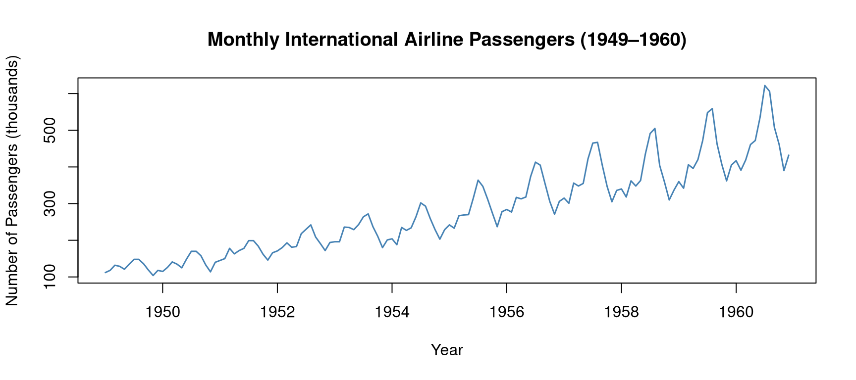
plot(AirPassengers,
     main = "Monthly International Airline Passengers (1949–1960)",
     ylab = "Number of Passengers (thousands)",
     xlab = "Year",
     col = "steelblue", lwd = 1.5)

Clearly shows an upward trend and growing seasonal pattern → multiplicative decomposition is appropriate.

Decomposition

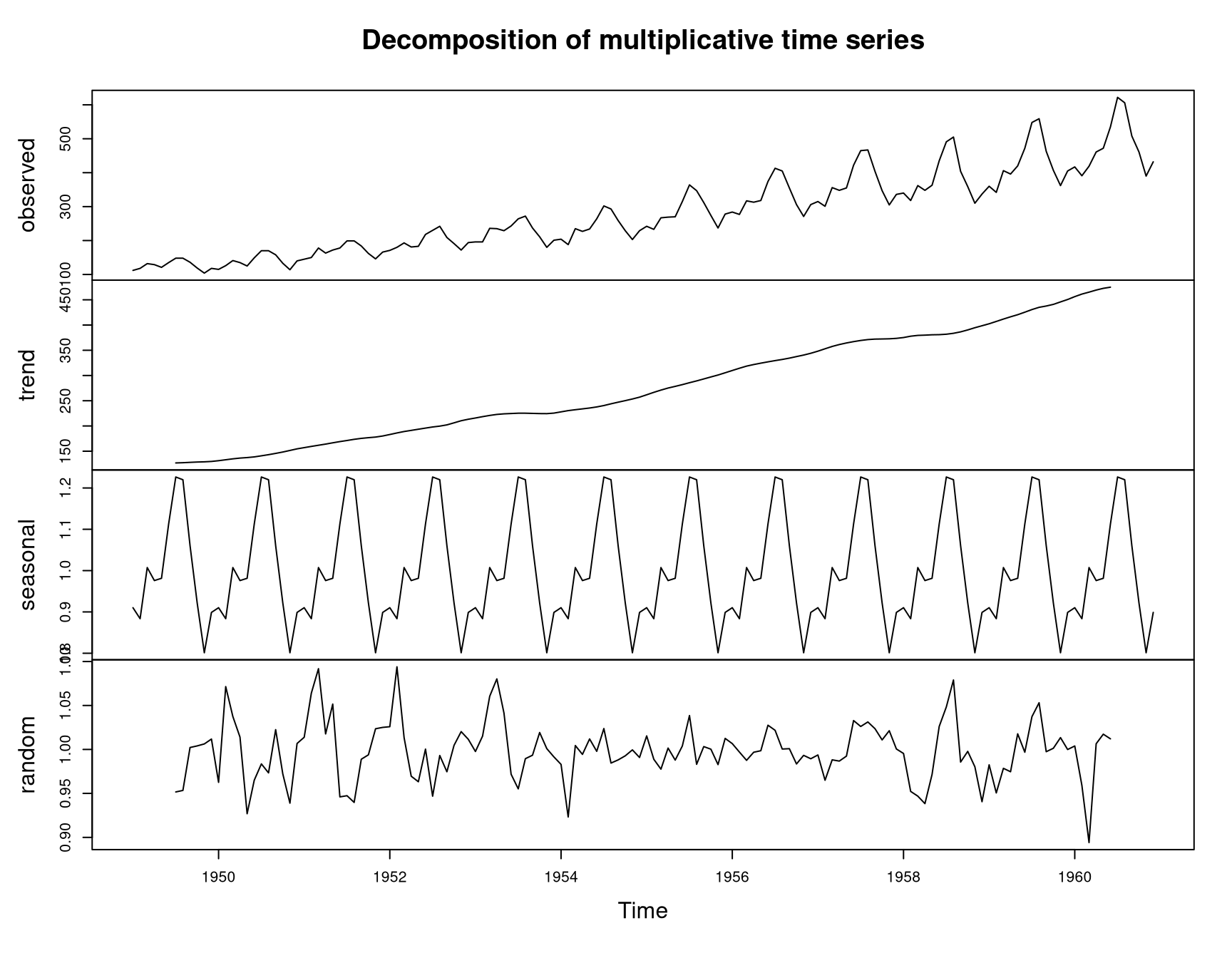
# Multiplicative decomposition (seasonal variation grows with level)
decomp <- decompose(AirPassengers, type = "multiplicative")
plot(decomp)

# View seasonal indices
round(decomp$seasonal[1:12], 4)
 [1] 0.9102 0.8836 1.0074 0.9759 0.9814 1.1128 1.2266 1.2199 1.0605 0.9218
[11] 0.8012 0.8988

Stationarity Testing — Augmented Dickey-Fuller Test

\[H_0: \text{Series has a unit root (non-stationary)}\] \[H_1: \text{Series is stationary}\]

# install.packages("tseries")
library(tseries)

adf.test(AirPassengers)

    Augmented Dickey-Fuller Test

data:  AirPassengers
Dickey-Fuller = -7.3186, Lag order = 5, p-value = 0.01
alternative hypothesis: stationary

If p-value > 0.05 → fail to reject \(H_0\) → series is non-stationary → need differencing.

ACF and PACF Plots

# Log-transform to stabilise variance, then first-difference
log_ap <- log(AirPassengers)
diff_log_ap <- diff(log_ap, differences = 1)

par(mfrow = c(1, 2))
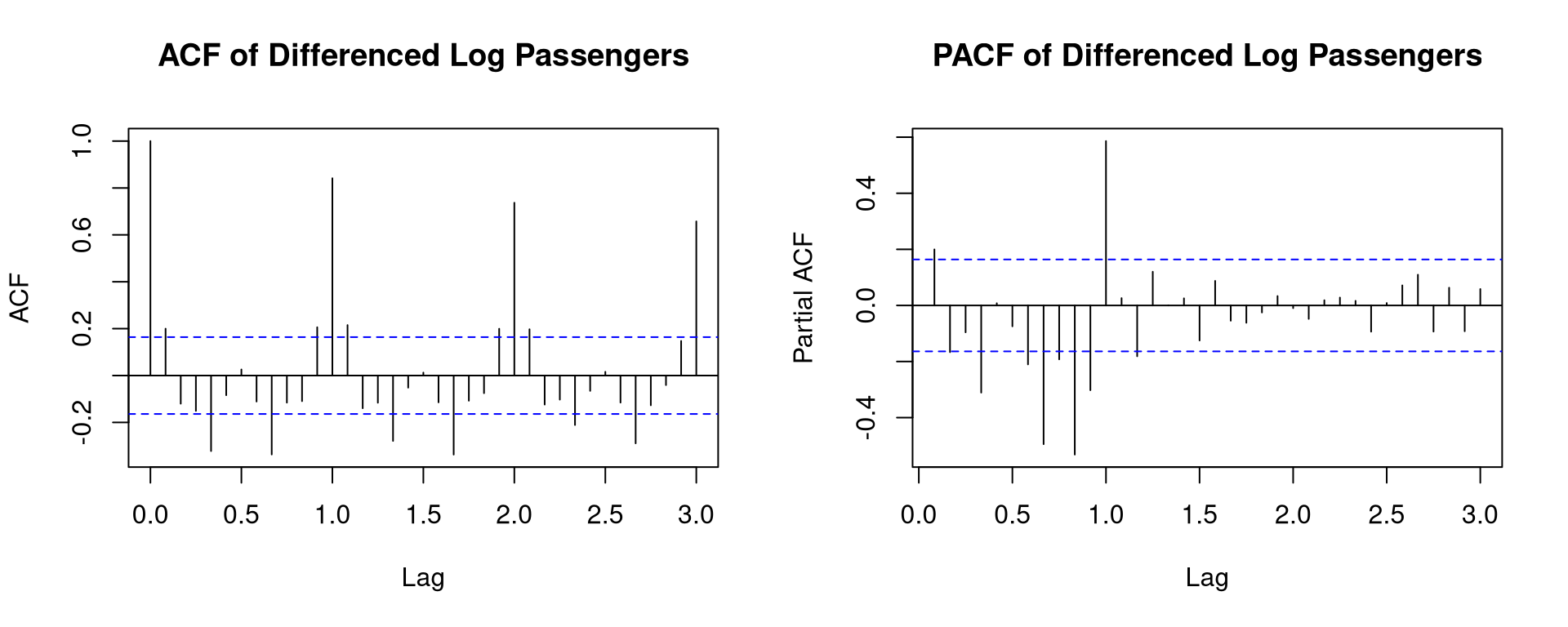
acf(diff_log_ap,  main = "ACF of Differenced Log Passengers",  lag.max = 36)
pacf(diff_log_ap, main = "PACF of Differenced Log Passengers", lag.max = 36)

Spikes at seasonal lags (12, 24) indicate seasonal ARIMA is needed.

Fitting ARIMA Model

# Manual ARIMA fit
model_arima <- arima(log_ap,
                     order = c(0, 1, 1),          # non-seasonal: d=1, MA(1)
                     seasonal = list(order = c(0, 1, 1), period = 12))

summary(model_arima)
          Length Class  Mode     
coef        2    -none- numeric  
sigma2      1    -none- numeric  
var.coef    4    -none- numeric  
mask        2    -none- logical  
loglik      1    -none- numeric  
aic         1    -none- numeric  
arma        7    -none- numeric  
residuals 144    ts     numeric  
call        4    -none- call     
series      1    -none- character
code        1    -none- numeric  
n.cond      1    -none- numeric  
nobs        1    -none- numeric  
model      10    -none- list     

Auto-ARIMA (automatic order selection)

# install.packages("forecast")
library(forecast)

model_auto <- auto.arima(AirPassengers, lambda = 0)  # lambda=0 for log transform
print(model_auto)
Series: AirPassengers 
ARIMA(0,1,1)(0,1,1)[12] 
Box Cox transformation: lambda= 0 

Coefficients:
          ma1     sma1
      -0.4018  -0.5569
s.e.   0.0896   0.0731

sigma^2 = 0.001371:  log likelihood = 244.7
AIC=-483.4   AICc=-483.21   BIC=-474.77

Forecasting

# Forecast 24 months ahead
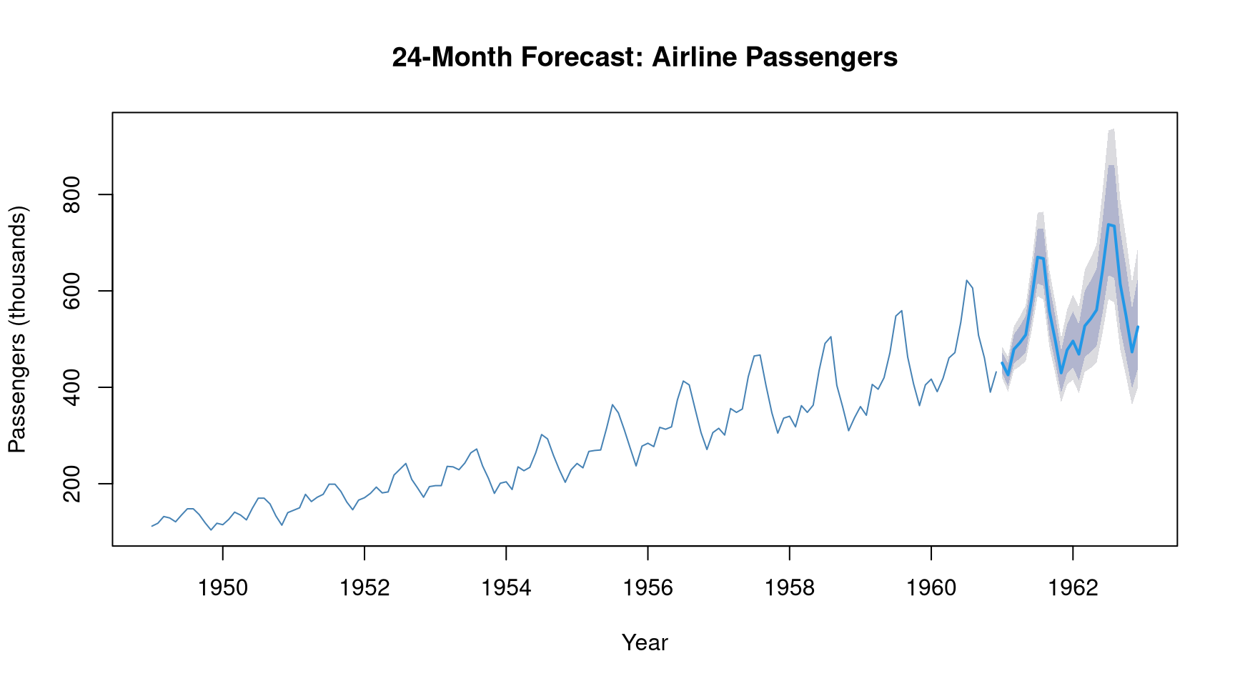
fc <- forecast(model_auto, h = 24)

plot(fc,
     main = "24-Month Forecast: Airline Passengers",
     ylab = "Passengers (thousands)",
     xlab = "Year",
     col = "steelblue")

# View forecast values with confidence intervals
print(fc)
         Point Forecast    Lo 80    Hi 80    Lo 95    Hi 95
Jan 1961       450.4224 429.5461 472.3132 418.8895 484.3289
Feb 1961       425.7172 402.8146 449.9219 391.1938 463.2874
Mar 1961       479.0068 450.1386 509.7265 435.5677 526.7781
Apr 1961       492.4045 459.8801 527.2290 443.5416 546.6503
May 1961       509.0550 472.7467 548.1518 454.5866 570.0497
Jun 1961       583.3449 538.8968 631.4591 516.7552 658.5155
Jul 1961       670.0108 615.9149 728.8579 589.0693 762.0740
Aug 1961       667.0776 610.3693 729.0546 582.3280 764.1613
Sep 1961       558.1894 508.4826 612.7552 483.9871 643.7679
Oct 1961       497.2078 451.0221 548.1230 428.3358 577.1537
Nov 1961       429.8720 388.3656 475.8144 368.0412 502.0903
Dec 1961       477.2426 429.4869 530.3083 406.1725 560.7482
Jan 1962       495.9301 441.4199 557.1717 415.0328 592.5957
Feb 1962       468.7289 414.3000 530.3084 388.0942 566.1170
Mar 1962       527.4025 463.0847 600.6535 432.2757 643.4631
Apr 1962       542.1538 473.0479 621.3551 440.1061 667.8634
May 1962       560.4865 486.1084 646.2450 450.8180 696.8336
Jun 1962       642.2823 553.8414 744.8460 512.0656 805.6127
Jul 1962       737.7043 632.5975 860.2747 583.1625 933.2006
Aug 1962       734.4748 626.4582 861.1161 575.8651 936.7700
Sep 1962       614.5852 521.4868 724.3039 478.0561 790.1058
Oct 1962       547.4424 462.1839 648.4284 422.5653 709.2234
Nov 1962       473.3034 397.6439 563.3587 362.6186 617.7735
Dec 1962       525.4600 439.3700 628.4185 399.6627 690.8531

Checking Residuals

# Residuals should look like white noise
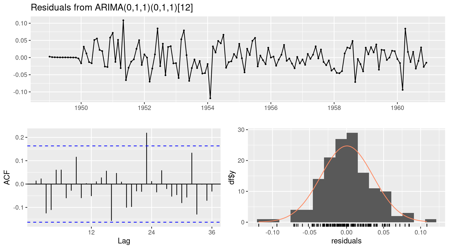
checkresiduals(model_auto)


    Ljung-Box test

data:  Residuals from ARIMA(0,1,1)(0,1,1)[12]
Q* = 26.446, df = 22, p-value = 0.233

Model df: 2.   Total lags used: 24

A good model leaves white noise residuals: - No autocorrelation in residuals - Residuals approximately normally distributed - Ljung-Box test p-value > 0.05

Accuracy Metrics

accuracy(model_auto)
                     ME     RMSE      MAE          MPE     MAPE     MASE
Training set 0.05140418 10.15504 7.357553 -0.004079016 2.623636 0.229706
                    ACF1
Training set -0.03689673
Metric Description
ME Mean Error
RMSE Root Mean Squared Error
MAE Mean Absolute Error
MAPE Mean Absolute Percentage Error
MASE Mean Absolute Scaled Error

Lower values = better model fit.

Exponential Smoothing (ETS) — Alternative Approach

model_ets <- ets(AirPassengers)
summary(model_ets)
ETS(M,Ad,M) 

Call:
ets(y = AirPassengers)

  Smoothing parameters:
    alpha = 0.7096 
    beta  = 0.0204 
    gamma = 1e-04 
    phi   = 0.98 

  Initial states:
    l = 120.9939 
    b = 1.7705 
    s = 0.8944 0.7993 0.9217 1.0592 1.2203 1.2318
           1.1105 0.9786 0.9804 1.011 0.8869 0.9059

  sigma:  0.0392

     AIC     AICc      BIC 
1395.166 1400.638 1448.623 

Training set error measures:
                   ME     RMSE      MAE       MPE     MAPE      MASE       ACF1
Training set 1.567359 10.74726 7.791605 0.4357799 2.857917 0.2432573 0.03945056
fc_ets <- forecast(model_ets, h = 24)
accuracy(fc_ets)
                   ME     RMSE      MAE       MPE     MAPE      MASE       ACF1
Training set 1.567359 10.74726 7.791605 0.4357799 2.857917 0.2432573 0.03945056

ETS models are often competitive with ARIMA and are simpler to interpret.


Summary

Concept Formula / Description R Function
Create ts object ts(data, start, frequency) ts()
Plot — plot()
Decompose \(Y_t = T_t + S_t + I_t\) decompose()
Stationarity test ADF test tseries::adf.test()
ACF / PACF \(\rho_k = \gamma_k / \gamma_0\) acf(), pacf()
Fit ARIMA \(\text{ARIMA}(p,d,q)\) arima()
Auto-fit — forecast::auto.arima()
Forecast — forecast()
Check residuals Ljung-Box test checkresiduals()

Time series analysis requires understanding the data’s structure — always plot first, decompose, check stationarity, then model.
© Pawan

Built with Quarto & R

  • Report an issue