Introduction
Regression analysis is a statistical method used to understand and quantify the relationship between variables . It helps us:
Explain how a dependent variable changes with one or more independent variables.
Predict future values of the dependent variable.
Example: How does a car’s fuel efficiency (MPG) change with its weight and horsepower?
Types of Regression
Simple Linear
Continuous
1 continuous
Multiple Linear
Continuous
2+ continuous/categorical
Logistic
Binary (0/1)
Any
Polynomial
Continuous
Powered terms
This paper focuses on Simple and Multiple Linear Regression .
Simple Linear Regression
Definition
Models the linear relationship between one predictor \(X\) and a response \(Y\) :
\[Y = \beta_0 + \beta_1 X + \varepsilon\]
where:
\(Y\) = dependent variable (response)\(X\) = independent variable (predictor)\(\beta_0\) = intercept (value of \(Y\) when \(X = 0\) )\(\beta_1\) = slope (change in \(Y\) per unit change in \(X\) )\(\varepsilon \sim N(0, \sigma^2)\) = random error term
Ordinary Least Squares (OLS) Estimation
OLS minimises the sum of squared residuals :
\[\text{SSR} = \sum_{i=1}^{n}(y_i - \hat{y}_i)^2 = \sum_{i=1}^{n}(y_i - \hat{\beta}_0 - \hat{\beta}_1 x_i)^2\]
The closed-form solutions are:
\[\hat{\beta}_1 = \frac{\sum_{i=1}^{n}(x_i - \bar{x})(y_i - \bar{y})}{\sum_{i=1}^{n}(x_i - \bar{x})^2} = \frac{S_{xy}}{S_{xx}}\]
\[\hat{\beta}_0 = \bar{y} - \hat{\beta}_1 \bar{x}\]
Goodness of Fit — R-squared
\[R^2 = 1 - \frac{\text{SSRes}}{\text{SST}} = 1 - \frac{\sum(y_i - \hat{y}_i)^2}{\sum(y_i - \bar{y})^2}\]
\(R^2 = 1\) : Perfect fit\(R^2 = 0\) : Model explains nothing\(0 < R^2 < 1\) : Proportion of variance explained
Multiple Linear Regression
Definition
\[Y = \beta_0 + \beta_1 X_1 + \beta_2 X_2 + \cdots + \beta_k X_k + \varepsilon\]
In matrix notation:
\[\mathbf{Y} = \mathbf{X}\boldsymbol{\beta} + \boldsymbol{\varepsilon}\]
OLS solution:
\[\hat{\boldsymbol{\beta}} = (\mathbf{X}^T\mathbf{X})^{-1}\mathbf{X}^T\mathbf{Y}\]
Adjusted R-squared
For multiple regression, use Adjusted \(R^2\) to penalise for extra predictors:
\[\bar{R}^2 = 1 - \frac{(1-R^2)(n-1)}{n-k-1}\]
where \(k\) = number of predictors and \(n\) = sample size.
Assumptions of Linear Regression (LINE)
L L inearity: relationship between \(X\) and \(Y\) is linear
I I ndependence: observations are independent
N N ormality: residuals are normally distributed
E E qual variance: residuals have constant variance (homoscedasticity)
When and Where to Use
Economics
Predicting GDP from investment and consumption
Medicine
Predicting blood pressure from age and BMI
Real estate
Predicting house price from area and location
Agriculture
Predicting crop yield from rainfall and temperature
HR analytics
Predicting salary from experience and education
Implementation in R
Simple Linear Regression
# Use mtcars: predict mpg from weight (wt) data (mtcars)# Fit the model <- lm (mpg ~ wt, data = mtcars)summary (model_simple)
Call:
lm(formula = mpg ~ wt, data = mtcars)

Residuals:
    Min      1Q  Median      3Q     Max
-4.5432 -2.3647 -0.1252  1.4096  6.8727

Coefficients:
            Estimate Std. Error t value Pr(>|t|)
(Intercept)  37.2851     1.8776  19.858  < 2e-16 ***
wt           -5.3445     0.5591  -9.559 1.29e-10 ***
---
Signif. codes:  0 '***' 0.001 '**' 0.01 '*' 0.05 '.' 0.1 ' ' 1

Residual standard error: 3.046 on 30 degrees of freedom
Multiple R-squared:  0.7528,    Adjusted R-squared:  0.7446
F-statistic: 91.38 on 1 and 30 DF,  p-value: 1.294e-10
Interpretation of Output
cat ("Intercept (β₀) :" , coef (model_simple)[1 ], " \n " )
Intercept (β₀) : 37.28513
cat ("Slope (β₁) :" , coef (model_simple)[2 ], " \n " )cat ("R-squared :" , summary (model_simple)$ r.squared, " \n " )cat ("Adj R-squared :" , summary (model_simple)$ adj.r.squared, " \n " )
Adj R-squared : 0.7445939
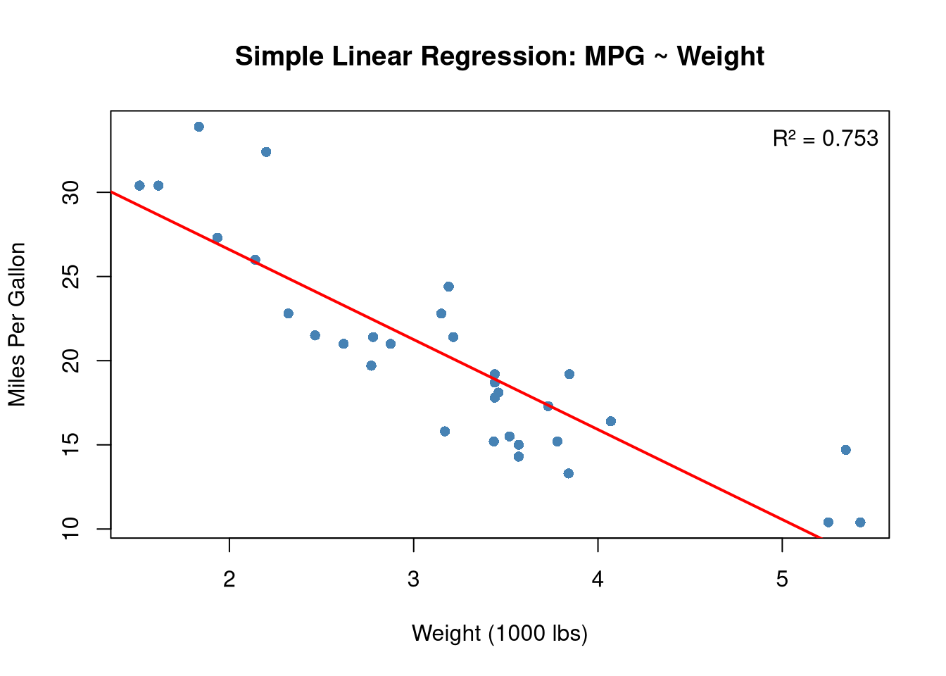
The slope of ~−5.34 means: for every 1000 lb increase in weight, MPG decreases by ~5.34.
Scatter Plot with Regression Line
plot (mtcars$ wt, mtcars$ mpg,pch = 16 , col = "steelblue" ,xlab = "Weight (1000 lbs)" ,ylab = "Miles Per Gallon" ,main = "Simple Linear Regression: MPG ~ Weight" )abline (model_simple, col = "red" , lwd = 2 )# Add R² label <- round (summary (model_simple)$ r.squared, 3 )legend ("topright" , legend = paste ("R² =" , r2), bty = "n" )
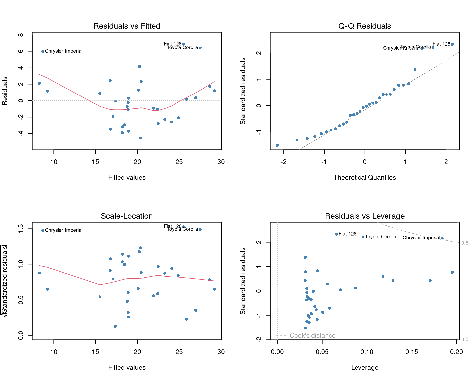
Residual Diagnostics
par (mfrow = c (2 , 2 ))plot (model_simple, col = "steelblue" , pch = 16 )
The four diagnostic plots check:
Residuals vs Fitted : Should show no pattern (linearity, homoscedasticity)Normal Q-Q : Points should follow the diagonal line (normality)Scale-Location : Should be horizontal (equal variance)Residuals vs Leverage : Identifies influential points
Multiple Linear Regression
# Predict mpg from weight AND horsepower <- lm (mpg ~ wt + hp, data = mtcars)summary (model_multi)
Call:
lm(formula = mpg ~ wt + hp, data = mtcars)

Residuals:
   Min     1Q Median     3Q    Max
-3.941 -1.600 -0.182  1.050  5.854

Coefficients:
            Estimate Std. Error t value Pr(>|t|)
(Intercept) 37.22727    1.59879  23.285  < 2e-16 ***
wt          -3.87783    0.63273  -6.129 1.12e-06 ***
hp          -0.03177    0.00903  -3.519  0.00145 **
---
Signif. codes:  0 '***' 0.001 '**' 0.01 '*' 0.05 '.' 0.1 ' ' 1

Residual standard error: 2.593 on 29 degrees of freedom
Multiple R-squared:  0.8268,    Adjusted R-squared:  0.8148
F-statistic: 69.21 on 2 and 29 DF,  p-value: 9.109e-12
cat ("Intercept :" , round (coef (model_multi)[1 ], 3 ), " \n " )cat ("β₁ (wt) :" , round (coef (model_multi)[2 ], 3 ), " \n " )cat ("β₂ (hp) :" , round (coef (model_multi)[3 ], 3 ), " \n " )cat ("Adjusted R² :" , round (summary (model_multi)$ adj.r.squared, 3 ), " \n " )
Compared to the simple model, adding horsepower increases Adjusted R² — meaning it adds explanatory power.
Comparing Models
# ANOVA test to compare models anova (model_simple, model_multi)
Analysis of Variance Table

Model 1: mpg ~ wt
Model 2: mpg ~ wt + hp
  Res.Df    RSS Df Sum of Sq      F   Pr(>F)
1     30 278.32
2     29 195.05  1    83.274 12.381 0.001451 **
---
Signif. codes:  0 '***' 0.001 '**' 0.01 '*' 0.05 '.' 0.1 ' ' 1
A significant p-value means the more complex model fits significantly better.
Prediction
# Predict MPG for a new car: wt = 3.0, hp = 110 <- data.frame (wt = 3.0 , hp = 110 )# Point prediction <- predict (model_multi, newdata = new_car)cat ("Predicted MPG:" , round (pred, 2 ), " \n " )# With 95% prediction interval <- predict (model_multi, newdata = new_car, interval = "prediction" )print (pred_interval)
       fit     lwr     upr
1 22.09875 16.6858 27.5117
Checking Multicollinearity (VIF)
# install.packages("car") library (car)vif (model_multi)
VIF < 5: No serious multicollinearity
VIF > 10: High multicollinearity — consider removing or combining predictors
Full Model with All Predictors
<- lm (mpg ~ ., data = mtcars)summary (model_full)$ adj.r.squared
# Stepwise selection to find the best model <- step (model_full, direction = "backward" , trace = 0 )summary (model_step)
Call:
lm(formula = mpg ~ wt + qsec + am, data = mtcars)

Residuals:
    Min      1Q  Median      3Q     Max
-3.4811 -1.5555 -0.7257  1.4110  4.6610

Coefficients:
            Estimate Std. Error t value Pr(>|t|)
(Intercept)   9.6178     6.9596   1.382 0.177915
wt           -3.9165     0.7112  -5.507 6.95e-06 ***
qsec          1.2259     0.2887   4.247 0.000216 ***
am            2.9358     1.4109   2.081 0.046716 *
---
Signif. codes:  0 '***' 0.001 '**' 0.01 '*' 0.05 '.' 0.1 ' ' 1

Residual standard error: 2.459 on 28 degrees of freedom
Multiple R-squared:  0.8497,    Adjusted R-squared:  0.8336
F-statistic: 52.75 on 3 and 28 DF,  p-value: 1.21e-11
Coefficient of Determination Summary
<- list ("Simple (wt only)" = model_simple,"Multiple (wt + hp)" = model_multi,"Stepwise selected" = model_step<- sapply (models, function (m) {c (R2 = round (summary (m)$ r.squared, 4 ),AdjR2 = round (summary (m)$ adj.r.squared, 4 ),AIC = round (AIC (m), 2 ))as.data.frame (t (results))
                       R2  AdjR2    AIC
Simple (wt only)   0.7528 0.7446 166.03
Multiple (wt + hp) 0.8268 0.8148 156.65
Stepwise selected  0.8497 0.8336 154.12
Summary
Fit model
\(Y = \beta_0 + \beta_1 X\) lm(Y ~ X)
View results
—
summary(model)
Coefficients
\(\hat{\boldsymbol{\beta}} = (\mathbf{X}^T\mathbf{X})^{-1}\mathbf{X}^T\mathbf{Y}\) coef(model)
Predict
\(\hat{y} = \hat{\beta}_0 + \hat{\beta}_1 x\) predict(model, newdata)
Diagnostics
—
plot(model)
VIF
—
car::vif(model)
Model comparison
—
anova(m1, m2), AIC()
Regression is the workhorse of statistical modelling. Always check assumptions via diagnostic plots before interpreting coefficients.