The Central Limit Theorem

The Most Important Theorem in Statistics

Introduction

The Central Limit Theorem (CLT) is arguably the most important result in all of statistics. It explains why the normal distribution appears everywhere in practice and forms the theoretical backbone of hypothesis testing, confidence intervals, and much of inferential statistics.

“No matter what shape the original population has, the distribution of the sample mean becomes approximately normal as the sample size increases.”

---

The Theorem — Formal Statement

Let \(X_1, X_2, \ldots, X_n\) be a random sample of size \(n\) drawn from any population with:

• Mean: \(\mu\)
• Finite variance: \(\sigma^2\)

Then as \(n \to \infty\), the distribution of the sample mean \(\bar{X}\) approaches a normal distribution:

\[\bar{X} \sim N\left(\mu,\ \frac{\sigma^2}{n}\right)\]

Or equivalently, the standardised sample mean:

\[Z = \frac{\bar{X} - \mu}{\sigma / \sqrt{n}} \xrightarrow{d} N(0, 1)\]

converges in distribution to the standard normal.

---

Key Components

Standard Error (SE)

The standard deviation of the sampling distribution of the mean is called the Standard Error:

\[SE = \frac{\sigma}{\sqrt{n}}\]

• As \(n\) increases → SE decreases → sample mean is more precise
• Doubling sample size reduces SE by factor of \(\sqrt{2} \approx 1.41\)

Rule of Thumb for Sample Size

Population Shape	Minimum \(n\) for CLT
Roughly symmetric	\(n \geq 30\)
Moderately skewed	\(n \geq 50\)
Heavily skewed / extreme outliers	\(n \geq 100\)

---

Why Is the CLT So Important?

1. Inference without knowing population distribution: We can build confidence intervals and run t-tests even when the population is not normal — as long as \(n\) is large enough.

2. Foundation of hypothesis testing: The Z-test and t-test are direct applications of the CLT.

3. Quality control: Manufacturing uses CLT to monitor process averages via control charts (X-bar charts).

4. Finance: Portfolio returns (averages of many individual stock returns) are approximately normal.

5. Polling and surveys: Sample proportions (a type of mean) follow a normal distribution for large samples.

---

When and Where to Use the CLT

Application	Description
Confidence intervals	\(\bar{x} \pm z_{\alpha/2} \cdot \frac{s}{\sqrt{n}}\)
One-sample Z-test	Test if population mean equals a value
Polling	Estimate proportions from survey data
Quality control (SPC)	Monitor sample means over time
Simulation / bootstrapping	Theoretical justification

---

Implementation in R

Simulating the CLT — Uniform Distribution

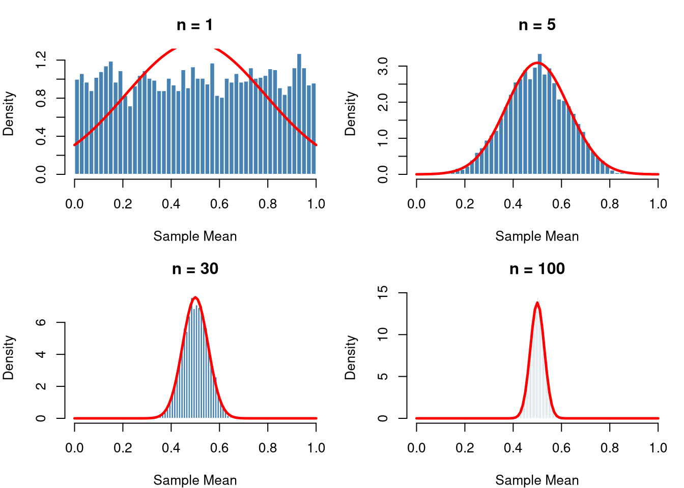
We draw repeated samples from a Uniform distribution (clearly non-normal) and watch the distribution of sample means converge to normal.

set.seed(42)

# Parameters
pop_mean <- 0.5   # mean of Uniform(0,1)
pop_sd   <- sqrt(1/12)  # sd of Uniform(0,1)

# Sample sizes to demonstrate
sample_sizes <- c(1, 5, 30, 100)
n_simulations <- 5000

par(mfrow = c(2, 2), mar = c(4, 4, 3, 1))

for (n in sample_sizes) {
  # Draw 5000 sample means, each from a sample of size n
  sample_means <- replicate(n_simulations, mean(runif(n, 0, 1)))

  hist(sample_means,
       breaks = 40,
       probability = TRUE,
       col = "steelblue",
       border = "white",
       main = paste("n =", n),
       xlab = "Sample Mean",
       xlim = c(0, 1))

  # Overlay the theoretical normal curve
  curve(dnorm(x, mean = pop_mean, sd = pop_sd / sqrt(n)),
        add = TRUE, col = "red", lwd = 2.5)
}

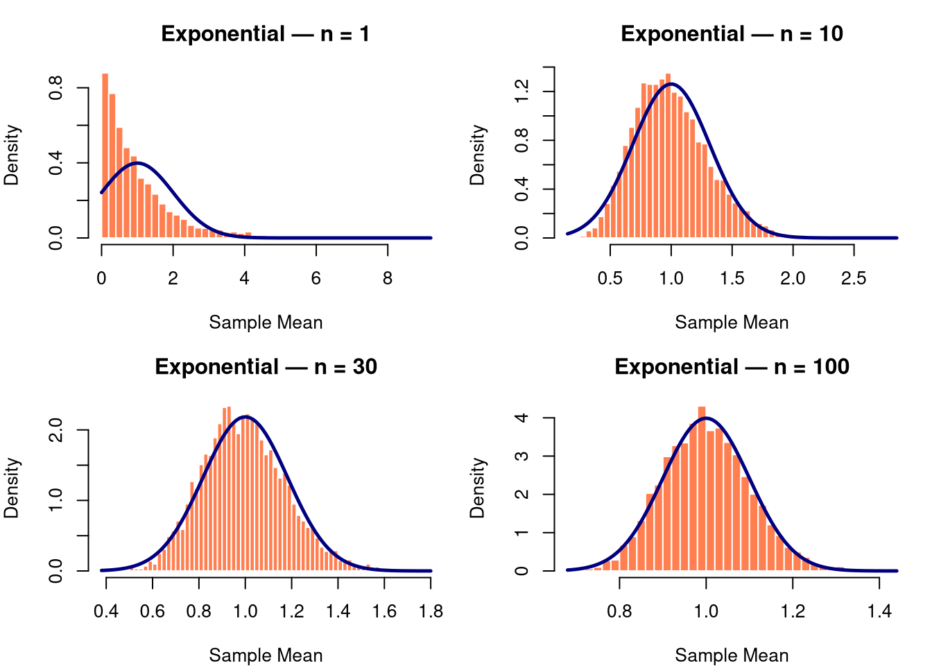
Simulating the CLT — Exponential Distribution (Very Skewed)

set.seed(123)

# Exponential with rate = 1: mean = 1, sd = 1
sample_sizes2 <- c(1, 10, 30, 100)

par(mfrow = c(2, 2), mar = c(4, 4, 3, 1))

for (n in sample_sizes2) {
  sample_means <- replicate(n_simulations, mean(rexp(n, rate = 1)))

  hist(sample_means,
       breaks = 50,
       probability = TRUE,
       col = "coral",
       border = "white",
       main = paste("Exponential — n =", n),
       xlab = "Sample Mean")

  # Theoretical normal overlay
  curve(dnorm(x, mean = 1, sd = 1 / sqrt(n)),
        add = TRUE, col = "navy", lwd = 2.5)
}

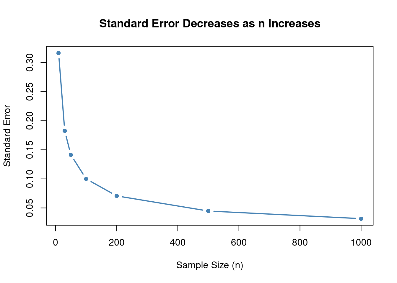
Demonstrating the Standard Error

# True SE shrinks as n increases
n_values <- c(10, 30, 50, 100, 200, 500, 1000)
true_se   <- 1 / sqrt(n_values)  # for Exp(1), sigma = 1

data.frame(
  n  = n_values,
  SE = round(true_se, 4)
)

     n     SE
1   10 0.3162
2   30 0.1826
3   50 0.1414
4  100 0.1000
5  200 0.0707
6  500 0.0447
7 1000 0.0316

plot(n_values, true_se,
     type = "b", pch = 16, col = "steelblue", lwd = 2,
     xlab = "Sample Size (n)",
     ylab = "Standard Error",
     main = "Standard Error Decreases as n Increases")
abline(h = 0, lty = 2, col = "grey")

Practical Application — Confidence Interval

Suppose we want to estimate the mean weight of students at a university. We take a sample of \(n = 50\) students.

set.seed(99)

# Simulated weight data (population: skewed, like real weight data)
weights <- rexp(50, rate = 1/70) + 40   # mean ≈ 110 lbs, shifted

n    <- length(weights)
xbar <- mean(weights)
s    <- sd(weights)
se   <- s / sqrt(n)

# 95% Confidence Interval using CLT (z = 1.96)
z    <- qnorm(0.975)
ci_lower <- xbar - z * se
ci_upper <- xbar + z * se

cat(sprintf("Sample Mean   : %.2f\n", xbar))

Sample Mean   : 116.07

cat(sprintf("Std Error     : %.2f\n", se))

Std Error     : 12.80

cat(sprintf("95%% CI        : (%.2f, %.2f)\n", ci_lower, ci_upper))

95% CI        : (90.98, 141.15)

The 95% CI means: if we repeated this sampling procedure 100 times, approximately 95 of those intervals would contain the true population mean.

Verifying Coverage Probability

set.seed(42)

# True mean = 70 (Exponential with rate=1/70, shifted)
true_mean <- 110
coverage_count <- 0
n_trials <- 1000
n_each <- 50

for (i in 1:n_trials) {
  samp <- rexp(n_each, rate = 1/70) + 40
  xbar_i <- mean(samp)
  se_i   <- sd(samp) / sqrt(n_each)
  lower  <- xbar_i - 1.96 * se_i
  upper  <- xbar_i + 1.96 * se_i
  if (lower <= true_mean && true_mean <= upper) {
    coverage_count <- coverage_count + 1
  }
}

cat(sprintf("Empirical coverage: %.1f%% (target: 95%%)\n",
            100 * coverage_count / n_trials))

Empirical coverage: 93.0% (target: 95%)

---

Summary

The Central Limit Theorem tells us:

1. Any population + large enough sample → sample mean is approximately normal
2. The sampling distribution centres at \(\mu\) with spread \(\sigma/\sqrt{n}\)
3. Larger \(n\) → smaller standard error → more precise estimates

Component	Formula	R function
Sample Mean	\(\bar{x} = \frac{\sum x_i}{n}\)	mean()
Standard Error	\(SE = s/\sqrt{n}\)	sd(x)/sqrt(n)
95% CI	\(\bar{x} \pm 1.96 \cdot SE\)	t.test(x)
Z-score	\(Z = (\bar{x} - \mu)/SE\)	manual computation
Normal quantile	\(z_{\alpha/2}\)	qnorm(0.975)

The CLT is why we can use normal-based methods on real-world data — even when the raw data is not normal.