Pawan.
  • About
  • Experience
  • Content Hub
  • Skills
  • Editor
  • R Code
  • Contact

On this page

  • Introduction
  • Key Concepts and Definitions
    • 1. Population vs Sample
    • 2. Measures of Central Tendency
      • Mean (Arithmetic Average)
      • Median
      • Mode
    • 3. Measures of Dispersion
      • Variance
      • Standard Deviation
      • Range
      • Interquartile Range (IQR)
    • 4. Measures of Shape
      • Skewness
      • Kurtosis
  • When and Where to Use Basic Statistics
  • Implementation in R
    • Loading and Exploring Data
    • Measures of Central Tendency
    • Measures of Dispersion
    • Quantiles and Summary
    • Skewness and Kurtosis
    • Full Descriptive Statistics Table
    • Visualisation
  • Interpretation
  • Summary
  • Report an issue

Other Formats

  • PDF

Basic Statistics

Concepts, Formulas, and Applications in R

Author

Pawan

Published

May 11, 2026

Introduction

Basic statistics is the foundation of all data analysis. It provides tools to summarize, describe, and understand data before performing any advanced modelling. It answers the most fundamental question: What does the data look like?


Key Concepts and Definitions

1. Population vs Sample

  • Population: The complete set of all items of interest (e.g., all students in India).
  • Sample: A subset of the population selected for study (e.g., 500 students from Delhi).

We use sample statistics to estimate population parameters.

Measure Population Symbol Sample Symbol
Mean μ (mu) x̄
Standard Deviation σ (sigma) s
Size N n

2. Measures of Central Tendency

These describe the centre of the data.

Mean (Arithmetic Average)

\[\bar{x} = \frac{\sum_{i=1}^{n} x_i}{n}\]

Median

The middle value when data is sorted. For \(n\) observations:

  • If \(n\) is odd: Median = \(\left(\frac{n+1}{2}\right)\)th value
  • If \(n\) is even: Median = average of \(\left(\frac{n}{2}\right)\)th and \(\left(\frac{n}{2}+1\right)\)th values

Mode

The value that occurs most frequently in the dataset.


3. Measures of Dispersion

These describe how spread out the data is.

Variance

\[s^2 = \frac{\sum_{i=1}^{n}(x_i - \bar{x})^2}{n-1}\]

Standard Deviation

\[s = \sqrt{\frac{\sum_{i=1}^{n}(x_i - \bar{x})^2}{n-1}}\]

Range

\[\text{Range} = x_{\max} - x_{\min}\]

Interquartile Range (IQR)

\[\text{IQR} = Q_3 - Q_1\]

where \(Q_1\) = 25th percentile and \(Q_3\) = 75th percentile.


4. Measures of Shape

Skewness

Measures asymmetry of the distribution.

\[\text{Skewness} = \frac{1}{n} \sum_{i=1}^{n} \left(\frac{x_i - \bar{x}}{s}\right)^3\]

  • Skewness = 0 → Symmetric
  • Skewness > 0 → Right-skewed (tail on the right)
  • Skewness < 0 → Left-skewed (tail on the left)

Kurtosis

Measures peakedness of the distribution.

\[\text{Kurtosis} = \frac{1}{n} \sum_{i=1}^{n} \left(\frac{x_i - \bar{x}}{s}\right)^4\]


When and Where to Use Basic Statistics

Situation Tool
Summarising exam scores Mean, Median, SD
Comparing income distributions Median, IQR (robust to outliers)
Understanding data shape Skewness, Kurtosis
Checking data spread Variance, Range
Exploratory Data Analysis (EDA) All of the above

Real-world examples: - A hospital computes the mean age of patients to plan resources. - An economist uses the median income (not mean) because income data is right-skewed. - A teacher computes standard deviation of marks to judge class variability.


Implementation in R

Loading and Exploring Data

# Use the built-in 'mtcars' dataset
data(mtcars)

# First look at the data
head(mtcars)
                   mpg cyl disp  hp drat    wt  qsec vs am gear carb
Mazda RX4         21.0   6  160 110 3.90 2.620 16.46  0  1    4    4
Mazda RX4 Wag     21.0   6  160 110 3.90 2.875 17.02  0  1    4    4
Datsun 710        22.8   4  108  93 3.85 2.320 18.61  1  1    4    1
Hornet 4 Drive    21.4   6  258 110 3.08 3.215 19.44  1  0    3    1
Hornet Sportabout 18.7   8  360 175 3.15 3.440 17.02  0  0    3    2
Valiant           18.1   6  225 105 2.76 3.460 20.22  1  0    3    1
str(mtcars)
'data.frame':   32 obs. of  11 variables:
 $ mpg : num  21 21 22.8 21.4 18.7 18.1 14.3 24.4 22.8 19.2 ...
 $ cyl : num  6 6 4 6 8 6 8 4 4 6 ...
 $ disp: num  160 160 108 258 360 ...
 $ hp  : num  110 110 93 110 175 105 245 62 95 123 ...
 $ drat: num  3.9 3.9 3.85 3.08 3.15 2.76 3.21 3.69 3.92 3.92 ...
 $ wt  : num  2.62 2.88 2.32 3.21 3.44 ...
 $ qsec: num  16.5 17 18.6 19.4 17 ...
 $ vs  : num  0 0 1 1 0 1 0 1 1 1 ...
 $ am  : num  1 1 1 0 0 0 0 0 0 0 ...
 $ gear: num  4 4 4 3 3 3 3 4 4 4 ...
 $ carb: num  4 4 1 1 2 1 4 2 2 4 ...

Measures of Central Tendency

# Focus on miles per gallon (mpg)
x <- mtcars$mpg

cat("Mean    :", mean(x), "\n")
Mean    : 20.09062 
cat("Median  :", median(x), "\n")
Median  : 19.2 
cat("Mode    :", as.numeric(names(sort(table(x), decreasing = TRUE)[1])), "\n")
Mode    : 10.4 

Measures of Dispersion

cat("Variance:", var(x), "\n")
Variance: 36.3241 
cat("Std Dev :", sd(x), "\n")
Std Dev : 6.026948 
cat("Range   :", range(x), "\n")
Range   : 10.4 33.9 
cat("IQR     :", IQR(x), "\n")
IQR     : 7.375 

Quantiles and Summary

# Five-number summary + mean
summary(x)
   Min. 1st Qu.  Median    Mean 3rd Qu.    Max. 
  10.40   15.43   19.20   20.09   22.80   33.90 
# Custom quantiles
quantile(x, probs = c(0.25, 0.50, 0.75, 0.90))
   25%    50%    75%    90% 
15.425 19.200 22.800 30.090 

Skewness and Kurtosis

# Install e1071 if not available: install.packages("e1071")
library(e1071)

cat("Skewness:", skewness(x), "\n")
Skewness: 0.610655 
cat("Kurtosis:", kurtosis(x), "\n")
Kurtosis: -0.372766 

Full Descriptive Statistics Table

# A clean descriptive statistics summary
desc_stats <- data.frame(
  Statistic = c("N", "Mean", "Median", "SD", "Variance",
                "Min", "Max", "Range", "IQR", "Skewness", "Kurtosis"),
  Value = round(c(
    length(x), mean(x), median(x), sd(x), var(x),
    min(x), max(x), diff(range(x)), IQR(x),
    skewness(x), kurtosis(x)
  ), 3)
)

print(desc_stats)
   Statistic  Value
1          N 32.000
2       Mean 20.091
3     Median 19.200
4         SD  6.027
5   Variance 36.324
6        Min 10.400
7        Max 33.900
8      Range 23.500
9        IQR  7.375
10  Skewness  0.611
11  Kurtosis -0.373

Visualisation

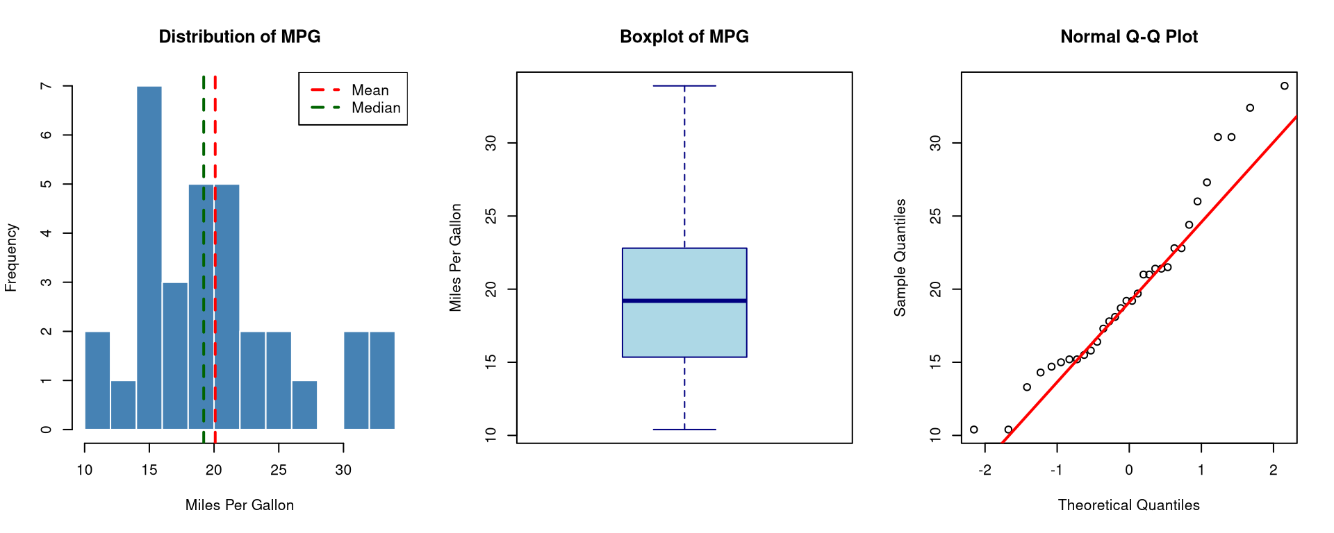
par(mfrow = c(1, 3))

# Histogram
hist(x,
     main = "Distribution of MPG",
     xlab = "Miles Per Gallon",
     col = "steelblue", border = "white",
     breaks = 10)
abline(v = mean(x), col = "red", lwd = 2, lty = 2)
abline(v = median(x), col = "darkgreen", lwd = 2, lty = 2)
legend("topright", legend = c("Mean", "Median"),
       col = c("red", "darkgreen"), lty = 2, lwd = 2)

# Boxplot
boxplot(x,
        main = "Boxplot of MPG",
        ylab = "Miles Per Gallon",
        col = "lightblue", border = "navy")

# QQ Plot (normality check)
qqnorm(x, main = "Normal Q-Q Plot")
qqline(x, col = "red", lwd = 2)


Interpretation

Looking at the MPG data from mtcars:

  • The mean MPG (~20.09) is slightly higher than the median (~19.2), suggesting a mild right skew.
  • The standard deviation (~6.03) tells us most cars fall within ±6 MPG of the mean.
  • The IQR spans from ~15.4 to ~22.8 MPG, covering the middle 50% of cars.
  • The Q-Q plot helps assess if the data follows a normal distribution.

Summary

Basic statistics transforms raw numbers into meaningful insights. Always start any data analysis by computing and visualising these descriptive measures — they guide every decision that follows.
What Formula R Function
Mean \(\bar{x} = \frac{\sum x_i}{n}\) mean()
Median Middle value median()
Variance \(s^2 = \frac{\sum(x_i - \bar{x})^2}{n-1}\) var()
Std Dev \(s = \sqrt{s^2}\) sd()
IQR \(Q_3 - Q_1\) IQR()
Summary All at once summary()

© Pawan

Built with Quarto & R

  • Report an issue